DP-600 Study Guide

Plan, implement, and manage a solution for data analytics (10–15%)
Plan a data analytics environment
When identifying requirements for a solution, it is crucial to consider various components and features that align with the business needs and objectives. Performance and capacity stock-keeping units (SKUs) also play a significant role in ensuring the solution can handle the expected workload. Here is a detailed explanation of these considerations:
Components and Features
- Components: Determine the necessary components of the solution, such as databases, storage systems, and networking resources. For instance, Azure SQL Database, Azure Synapse Analytics, or Azure Cosmos DB might be required depending on the data workloads.
- Features: Identify the specific features needed to meet the solution’s objectives. This could include data security features, such as encryption and access controls, or data integration and management features, like data streaming and batch processing capabilities https://learn.microsoft.com/en-us/industry/manufacturing/appendix/microsoft-technology .
Performance
- Performance Requirements: Assess the performance needs by considering the volume of transactions, query performance, and data processing speeds. This involves understanding the latency requirements and throughput for the application.
- Tuning and Optimization: Consider the ability to tune and optimize the solution for better performance. Azure services often provide tools and services for performance monitoring and tuning.
Capacity Stock-Keeping Units (SKUs)
- SKU Selection: Choose the right SKU that matches the performance and capacity needs of the solution. Azure offers a variety of compute SKUs, including memory-optimized, CPU-optimized, and general-purpose options https://learn.microsoft.com/en-us/industry/manufacturing/appendix/microsoft-technology .
- Scalability: Ensure that the selected SKUs provide scalability options to accommodate future growth. This includes autoscaling features and the ability to upgrade to higher SKUs as needed.
- Cost Considerations: Balance the performance and capacity requirements with cost. Selecting the appropriate SKU can help optimize costs by avoiding over-provisioning and under-provisioning of resources.
For additional information on Azure services and SKUs, you can refer to the following resources: - Azure SQL Database - Azure Synapse Analytics - Azure Cosmos DB - Azure Compute SKUs
By carefully considering these aspects, you can ensure that the solution is well-equipped to meet the current and future demands of the business.
Plan, implement, and manage a solution for data analytics (10–15%)
Implement and manage a data analytics environment
Implementing Workspace and Item-Level Access Controls for Fabric Items
When managing access to Fabric items, it is essential to understand the concepts of workspaces and item-level access controls. Here’s a detailed explanation of how to implement these controls:
Workspace-Level Access Controls
Workspaces in Fabric are collections of related data items that facilitate collaboration by grouping functionality in a single environment. To manage access at the workspace level:
Assign Workspace Roles: Fabric provides different workspace roles that determine the level of access users have. These roles include:
- Viewer: A read-only role allowing users to query data but not create or write data.
- Admin, Member, and Contributor: Read-write roles that enable users to view, create, manage, and write data to items within the workspace https://learn.microsoft.com/en-us/fabric/onelake/get-started-security .
Manage Workspace Permissions: As a workspace admin, you can grant or revoke workspace roles to control who can access the data. This is done by assigning roles to users or security groups within the organization https://learn.microsoft.com/en-us/fabric/admin/admin-overview .
Use Security Groups: By assigning workspace roles to security groups, you can simplify the management of access controls. Adding or removing members from the security group updates their access to the workspace accordingly https://learn.microsoft.com/en-us/fabric/onelake/get-started-security .
Item-Level Access Controls
Item-level access controls allow for more granular management of individual Fabric items such as apps, lakehouses, warehouses, and reports.
Create and Share Items: On the Home page, you can create and share items. The items you see are determined by the permissions granted to you across various workspaces https://learn.microsoft.com/en-us/fabric/get-started/fabric-home .
Control Access to Items: When you create an item, you can specify who has access to it. This control is separate from workspace-level roles and can be adjusted per item https://learn.microsoft.com/en-us/fabric/get-started/fabric-terminology .
Navigate to Workspaces: To manage item-level access, navigate to the specific workspace where the item resides. Use the Explorer pane to select the workspace and view the items you have permissions to access https://learn.microsoft.com/en-us/fabric/get-started/onelake-data-hub .
Understand Capacity: Capacity refers to the dedicated resources available for use. It is important to note that different items consume different capacities. Managing capacity is a part of controlling access to items, as it defines the ability of a resource to perform activities or produce output https://learn.microsoft.com/en-us/fabric/get-started/fabric-terminology .
For more information on managing workspaces and item-level access controls, refer to the following resources: - Workspaces and Roles - What is Capacity? - Workspaces Article
By implementing these workspace and item-level access controls, you can ensure that Fabric items are securely managed and that only authorized users have the appropriate level of access.
Plan, implement, and manage a solution for data analytics (10–15%)
Implement and manage a data analytics environment
Implementing Data Sharing for Workspaces, Warehouses, and Lakehouses
Data sharing in Azure is a critical aspect of collaborative data science and analytics. It involves configuring permissions and settings to allow secure access to data resources such as workspaces, warehouses, and lakehouses. Below is a detailed explanation of how to implement data sharing for these resources.
Workspaces
Workspaces in Azure are collaborative environments where teams can work on various data and analytics services. To share a workspace, you need to manage workspace roles, which apply to all items within it. These roles can include Owner, Contributor, Reader, and others, each with different levels of access and permissions. It’s important to assign these roles carefully to ensure that team members have the appropriate access levels for their tasks.
For more information on workspace roles and permissions, refer to the Azure RBAC documentation: Azure Role-Based Access Control (RBAC).
Warehouses
Warehouses in Azure, such as those in Microsoft Fabric, offer an easy experience to create reports and manage data. Sharing a warehouse allows users to build content based on the underlying default Power BI semantic model, query data using SQL, or access underlying data files. The context menu in the warehouse provides options such as ‘Open’, ‘Share’, ‘Analyze in Excel’, ‘Create report’, and ‘Manage permissions’. Each option is designed to facilitate different aspects of data sharing and collaboration.
To share a warehouse, you can use the ‘Share’ option, which lets you share warehouse access with other users in your organization. Users receive an email with links to access the detail page, where they can find the SQL connection string and access the default semantic model to create reports based on it.
For a detailed guide on sharing warehouses and managing permissions, see: Share your warehouse and manage permissions.
Lakehouses
Lakehouses are a new paradigm that combines the features of data lakes and data warehouses. Sharing data in a lakehouse involves setting up permissions at the file and folder level within the data lake storage, as well as managing access to the data warehouse layer built on top of it. In Azure, this can be done using Azure Synapse Analytics, which allows you to manage access to both SQL resources and the underlying data lake storage.
For SQL resources within Azure Synapse workspaces, you can create custom Azure roles for labeling and data classification as needed. This ensures that only authorized users can read or modify the data classification of a database.
For more information on creating custom roles and managing data classification in Azure Synapse Analytics, refer to the Microsoft.Synapse documentation: Microsoft.Synapse.
Additional Considerations
When implementing data sharing, it’s essential to consider the security and compliance requirements of your organization. Ensure that all shared data is protected and that users have access only to the data they are authorized to view or modify. Regularly review and update permissions to maintain a secure data sharing environment.
By following these guidelines and utilizing the provided resources, you can effectively implement data sharing for workspaces, warehouses, and lakehouses in Azure, facilitating collaboration while maintaining data security and governance.
Plan, implement, and manage a solution for data analytics (10–15%)
Implement and manage a data analytics environment
Manage Sensitivity Labels in Semantic Models and Lakehouses
Sensitivity labels are a critical feature in data governance and compliance, providing a mechanism to classify and protect sensitive data. When managing sensitivity labels in semantic models and lakehouses, it is essential to understand how these labels can be applied, inherited, and maintained to ensure data security.
Inheritance of Sensitivity Labels
Power BI semantic models that connect to sensitivity-labeled data in supported data sources can inherit those labels. This means that when data is brought into Power BI, it retains its classification, helping to keep the data secure within the Power BI environment https://learn.microsoft.com/en-us/fabric/admin/service-admin-portal-information-protection .
Applying Sensitivity Labels
To apply sensitivity labels to your data, you must have the appropriate permissions. In the context of Microsoft Fabric items, sensitivity labels from Microsoft Purview Information Protection can be used to protect sensitive content from unauthorized access and data leakage. These labels are a key part of meeting governance and compliance requirements for your organization https://learn.microsoft.com/en-us/fabric/get-started/apply-sensitivity-labels .
Requirements for Applying Labels
To apply sensitivity labels to Fabric items, you need:
- A Power BI Pro or Premium Per User (PPU) license.
- Edit permissions on the item you wish to label https://learn.microsoft.com/en-us/fabric/get-started/apply-sensitivity-labels .
If you are unable to apply a sensitivity label, or if the label is greyed out, it may be due to a lack of permissions to use that label. In such cases, contact your organization’s tech support https://learn.microsoft.com/en-us/fabric/get-started/apply-sensitivity-labels .
Exporting Items with Sensitivity Labels
When exporting items from Fabric, sensitivity labels are not included. Administrators have the option to block the export of items with sensitivity labels or to allow the export without the labels https://learn.microsoft.com/en-us/fabric/admin/git-integration-admin-settings .
Programmatically Managing Sensitivity Labels
For advanced management, you can use the REST API to manage classifications and recommendations programmatically. The REST API supports operations such as creating or updating sensitivity labels, deleting labels, enabling or disabling recommendations, and listing current or recommended labels for a database https://learn.microsoft.com/en-us/azure/azure-sql/database/data-discovery-and-classification-overview .
Additional Resources
For more information on sensitivity label inheritance from data sources, you can refer to the following resource: - Sensitivity label inheritance from data sources (preview).
To learn how to apply sensitivity labels in Power BI Desktop, visit: - Apply sensitivity labels in Power BI Desktop.
For a visual guide on sensitivity labels in the Fabric admin settings, see: - Sensitivity labels in Fabric admin settings.
For details on the REST API operations related to sensitivity labels, explore: - REST API for sensitivity labels.
By understanding and utilizing these features, you can effectively manage sensitivity labels in semantic models and lakehouses, ensuring that your data remains secure and compliant with organizational policies.
Plan, implement, and manage a solution for data analytics (10–15%)
Implement and manage a data analytics environment
Configure Fabric-Enabled Workspace Settings
When configuring Fabric-enabled workspace settings, it is essential to understand the various options available to optimize the workspace for different scenarios. Here are the key settings that can be configured:
High Concurrency Mode
High concurrency mode is a feature that allows multiple users to execute Spark jobs simultaneously without significant wait times. To configure this setting:
- Go to Workspace Settings.
- Under the Synapse section, select Spark Compute.
- Find the High Concurrency section where you can enable or disable this feature.
- Enabling high concurrency allows users to start or attach to a high concurrency session in their notebooks.
- Disabling it will hide the options related to configuring the time period of inactivity and starting new high concurrency sessions https://learn.microsoft.com/en-us/fabric/data-science/../data-engineering/configure-high-concurrency-session-notebooks .
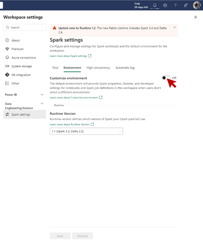
Environment Configuration
Configuring the environment is crucial for managing the workspace’s data engineering and science settings:
- Navigate to Workspace settings -> Data Engineering/Science -> Environment.
- Select Enable environment to remove existing configurations and start with a fresh workspace-level environment setup.
- Toggle Customize environment to the On position to attach an environment as a workspace default.
- Choose the previously configured environment as the workspace default and select Save.
- Confirm that the new environment appears under Default environment for workspace on the Spark settings page https://learn.microsoft.com/en-us/fabric/data-science/../data-engineering/environment-workspace-migration .
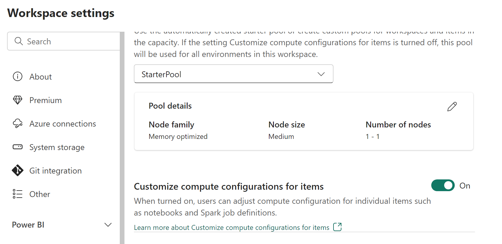
Fabric Environment Preview
The Fabric environment feature, currently in preview, allows workspace admins to:
- Enable or disable compute customizations in the Pool tab under Data Engineering/Science in Workspace settings.
- Delegate members and contributors to change default session-level compute configurations.
- Configure Spark session level properties to customize memory and cores of executors based on workload requirements https://learn.microsoft.com/en-us/fabric/data-engineering/environment-manage-compute .
Domain Management Settings
Domain management settings control the ability of tenant and domain admins to manage workspace domain assignments:
- Access the Admin portal.
- Go to Tenant settings > Domain management settings.
- Expand Allow tenant and domain admins to override workspace assignments (preview).
- Set the toggle to enable or disable the setting as required https://learn.microsoft.com/en-us/fabric/admin/service-admin-portal-domain-management-settings .
Power BI Integration with Azure Log Analytics
For monitoring and analytics, Power BI integration with Azure Log Analytics can be configured:
- Ensure the switch for Azure Log Analytics integration is turned on.
- Administrators and Premium workspace owners can then configure Azure Log Analytics for Power BI https://learn.microsoft.com/en-us/fabric/admin/service-admin-portal-audit-usage .
For additional information and detailed steps on configuring these settings, you can refer to the following URLs:
- High Concurrency Mode: High Concurrency Mode for Notebooks
- Environment Configuration: Environment Migration
- Fabric Environment Preview: Customize Compute Configurations
- Domain Management Settings: Domain REST APIs
- Power BI Integration: Azure Log Analytics for Power BI
By carefully configuring these settings, you can tailor the Fabric-enabled workspace to meet the specific needs of your data engineering and data science projects.
Plan, implement, and manage a solution for data analytics (10–15%)
Implement and manage a data analytics environment
Manage Fabric Capacity
Managing Fabric capacity is a critical aspect of optimizing and controlling costs for data warehousing and analytics workloads in Microsoft Fabric. Here’s a detailed explanation of the key points related to managing Fabric capacity:
Understanding Fabric Capacity Usage
- Compute Usage Reporting: It’s essential to monitor the compute usage of the Synapse Data Warehouse in Microsoft Fabric, which includes both read and write activity against the Warehouse and read activity on the SQL analytics endpoint of the Lakehouse. Usage charges are visible in the Azure portal under your subscription in Microsoft Cost Management https://learn.microsoft.com/en-us/fabric/data-warehouse/usage-reporting .
- Billing Insights: To gain a deeper understanding of your Fabric billing, you can refer to the documentation on understanding your Azure bill on a Fabric capacity https://learn.microsoft.com/en-us/fabric/data-warehouse/usage-reporting .
Cost Management
- Pausing Fabric Capacity: To save costs, Microsoft Fabric capacity can be paused when not in use. This action affects the Synapse Data Warehouse, as it cannot be paused individually. Pausing the entire Fabric capacity is a strategic move to manage expenses https://learn.microsoft.com/en-us/fabric/data-warehouse/pause-resume .
- Resuming Fabric Capacity: After pausing, you can resume your Fabric capacity as needed. The documentation provides guidance on how to pause and resume your Fabric capacity effectively https://learn.microsoft.com/en-us/fabric/data-warehouse/pause-resume .
Performance and Optimization
- Throttling and Smoothing: To maintain optimal performance, it’s important to understand the concepts of throttling and smoothing within Fabric Data Warehousing. Throttling ensures that no single workload monopolizes resources, while smoothing allows for the distribution of compute capacity over a 24-hour window to prevent immediate throttling https://learn.microsoft.com/en-us/fabric/data-factory/../get-started/whats-new https://learn.microsoft.com/en-us/fabric/data-warehouse/compute-capacity-smoothing-throttling .
- SSD Caching: Local SSD caching is a feature that stores frequently accessed data on local disks in a highly optimized format, which can significantly reduce I/O latency and improve performance https://learn.microsoft.com/en-us/fabric/data-factory/../get-started/whats-new .
Security and Compliance
- Column-level & Row-level Security: Fabric Warehouse and SQL analytics endpoint now support column-level and row-level security features, which are in preview. These features provide granular control over data access and are similar to those available in SQL Server https://learn.microsoft.com/en-us/fabric/data-factory/../get-started/whats-new .
Utilization and Billing Reporting
- Utilization Reporting: Utilization and billing reporting for Fabric data warehousing is available in the Microsoft Fabric Capacity Metrics app. This tool helps you track and manage your data warehousing utilization and associated costs https://learn.microsoft.com/en-us/fabric/data-factory/../get-started/whats-new https://learn.microsoft.com/en-us/fabric/data-warehouse/compute-capacity-smoothing-throttling .
Additional Resources
- Overages: The Overages tab in the Microsoft Fabric Capacity Metrics app provides a visual history of any overutilization of capacity, including details on carry forward, cumulative, and burndown of utilization https://learn.microsoft.com/en-us/fabric/data-warehouse/compute-capacity-smoothing-throttling .
- Related Documentation: For more comprehensive information on managing Fabric capacity, you can explore related content on billing and utilization reporting, performance guidelines, and burstable capacity in Fabric data warehousing https://learn.microsoft.com/en-us/fabric/data-warehouse/compute-capacity-smoothing-throttling .
For further reading and to access additional resources, please visit the following URLs: - Understand your Azure bill on a Fabric capacity https://learn.microsoft.com/en-us/fabric/data-warehouse/usage-reporting . - Pause and resume your capacity https://learn.microsoft.com/en-us/fabric/data-warehouse/pause-resume . - Throttling in Microsoft Fabric https://learn.microsoft.com/en-us/fabric/data-warehouse/compute-capacity-smoothing-throttling . - Overages in the Microsoft Fabric Capacity Metrics app https://learn.microsoft.com/en-us/fabric/data-warehouse/compute-capacity-smoothing-throttling . - Synapse Data Warehouse in Microsoft Fabric performance guidelines https://learn.microsoft.com/en-us/fabric/data-warehouse/compute-capacity-smoothing-throttling . - Burstable capacity in Fabric data warehousing https://learn.microsoft.com/en-us/fabric/data-warehouse/compute-capacity-smoothing-throttling . - Pause and resume in Fabric data warehousing https://learn.microsoft.com/en-us/fabric/data-warehouse/compute-capacity-smoothing-throttling .
By understanding and effectively managing Fabric capacity, organizations can ensure that their data warehousing and analytics workloads are running efficiently while also controlling costs.
Plan, implement, and manage a solution for data analytics (10–15%)
Manage the analytics development lifecycle
Implementing Version Control for a Workspace
Version control is a critical aspect of managing changes and maintaining the integrity of projects within a workspace. It allows developers to track modifications, collaborate efficiently, and revert to previous states when necessary. In the context of Microsoft Fabric, implementing version control for a workspace can be achieved through the integration of git, a widely-used version control system.
Git Integration in Microsoft Fabric
Microsoft Fabric has introduced git integration to provide seamless source control management. This feature enables developers to:
- Backup and Version Work: Developers can save snapshots of their work at different stages, creating a history of changes that can be reviewed or restored.
- Rollback Capabilities: If a new change introduces issues, developers can easily revert to a previous version that worked correctly.
- Collaboration and Isolation: Team members can work together on the same project or independently using git branches, which allows for isolated changes that can be merged later.
Connecting the Workspace to an Azure Repo
To implement version control in a Microsoft Fabric workspace, you need to connect the workspace to an Azure repository. The process involves the following steps:
Setting Up Azure Repos: Before integrating git into your Fabric workspace, you need to have an Azure repo ready to use. Azure Repos provides Git repositories or Team Foundation Version Control (TFVC) for source control of your code.
Integrating Git with Fabric Workspace: Once you have your Azure repo, you can integrate it with your Fabric workspace. This allows you to commit changes to your repo directly from the Fabric environment.
Versioning Workflows: With git integration, you can adopt various versioning workflows such as feature branching, forking, and pull requests. These workflows facilitate better management of features and contributions, ensuring that the main codebase remains stable.
Collaboration and Code Reviews: Git integration supports collaboration among team members. Code reviews can be conducted through pull requests, ensuring that code is reviewed and approved before it is merged into the main branch.
For more detailed guidance on integrating git with Microsoft Fabric, you can refer to the following resources:
- Introducing git integration in Microsoft Fabric for seamless source control management.
- Connecting the workspace to an Azure repo.
By following these steps and utilizing the provided resources, you can effectively implement version control for your workspace in Microsoft Fabric, ensuring a robust and collaborative development process https://learn.microsoft.com/en-us/fabric/get-started/whats-new-archive .
Plan, implement, and manage a solution for data analytics (10–15%)
Manage the analytics development lifecycle
Create and Manage a Power BI Desktop Project (.pbip)
A Power BI Desktop project, identified by the .pbip file
extension, is a specialized file format used by advanced content
creators for complex data model and report management scenarios. Unlike
a .pbix or .pbit file, a .pbip
project file does not contain any data. Instead, it serves as a
framework for sharing common model patterns, such as date tables, DAX
measure expressions, or calculation groups, which can save significant
development time https://learn.microsoft.com/power-bi/guidance/fabric-adoption-roadmap-mentoring-and-user-enablement
.
Creating a Power BI Desktop Project
To create a Power BI Desktop project, you can use Power BI Desktop in
developer mode. This mode allows for advanced editing and authoring,
which can be done in code editors like Visual Studio Code. Here are the
steps to create a .pbip file:
- Open Power BI Desktop in developer mode.
- Design your data model by defining tables, relationships, measures, and any other model patterns you wish to include.
- Save your work as a
.pbipfile, which can then be shared with other developers or content creators.
Managing a Power BI Desktop Project
Managing a .pbip project involves several advanced
practices that facilitate collaboration and version control:
Separation of Concerns:
.pbipfiles allow for a clear separation between the semantic model and report items, enabling multiple developers to work on different aspects of the project simultaneously https://learn.microsoft.com/power-bi/guidance/fabric-adoption-roadmap-mentoring-and-user-enablement .Source Control Integration: Power BI project files can be integrated with source control systems like Fabric Git, which helps in tracking changes and managing versions of the project https://learn.microsoft.com/power-bi/guidance/fabric-adoption-roadmap-mentoring-and-user-enablement .
Continuous Integration and Delivery (CI/CD): By using CI/CD techniques, teams can automate the integration, testing, and deployment of changes or new versions of the project content https://learn.microsoft.com/power-bi/guidance/fabric-adoption-roadmap-mentoring-and-user-enablement .
Additional Resources
For more information on creating and managing Power BI Desktop projects, you can refer to the following resources:
- Power BI Project Overview https://learn.microsoft.com/power-bi/guidance/fabric-adoption-roadmap-mentoring-and-user-enablement
- Advanced Data Model Management https://learn.microsoft.com/power-bi/guidance/fabric-adoption-roadmap-mentoring-and-user-enablement
- Power BI Desktop Developer Mode https://learn.microsoft.com/power-bi/guidance/fabric-adoption-roadmap-mentoring-and-user-enablement
By utilizing .pbip files and the associated best
practices, Power BI developers can enhance their productivity, maintain
high standards of quality, and ensure that their projects are robust and
easily maintainable.
Plan, implement, and manage a solution for data analytics (10–15%)
Manage the analytics development lifecycle
Plan and Implement Deployment Solutions
When planning and implementing deployment solutions, it is essential to consider the various services and tools provided by Microsoft to streamline the process. Here’s a detailed explanation of key points to consider:
Microsoft Cloud Solution Center
The Microsoft Cloud Solution Center is a centralized platform for deploying and configuring Microsoft industry cloud solutions. It offers a unified view of industry cloud capabilities and simplifies the deployment process across Microsoft 365, Azure, Dynamics 365, and Power Platform. The Solution Center assists with checking licensing requirements and dependencies, ensuring that all necessary components are in place for deployment https://learn.microsoft.com/en-us/industry/healthcare/../solution-center-deploy .
Data Encryption and Sovereignty
For customers with data sovereignty concerns, particularly those implementing Microsoft Cloud for Sovereignty, data encryption is a critical consideration. Key management in the cloud is a vital part of this process. Planning for encryption at the platform level involves identifying key management requirements, making technology choices, and selecting designs for Azure services. This planning is crucial for customers who need to comply with strict data sovereignty requirements https://learn.microsoft.com/en-us/industry/sovereignty/customer-managed-keys .
Business Continuity and Disaster Recovery
Azure Cosmos DB for MongoDB vCore requires a well-thought-out disaster recovery plan to maintain business continuity and prepare for potential service outages. Planning for high availability and initiating failover to another Azure region are critical steps in this process. Azure Cosmos DB for MongoDB vCore provides automatic backups without impacting database performance, which are retained for different intervals depending on the cluster’s status https://learn.microsoft.com/en-AU/azure/cosmos-db/mongodb/vcore/failover-disaster-recovery .
Deployment Using Templates
Templates can be used to deploy a group of Azure Logic Apps, such as those that ingest FHIR data into Dataverse healthcare APIs or Azure Health Data Services. The Azure Resource Manager (ARM) template titled “Healthcare data pipeline template” is available for deployment and provides a robust solution for enterprise-level data processing. Post-deployment, the Logic Apps can be customized to meet specific system needs https://learn.microsoft.com/dynamics365/industry/healthcare/dataverse-healthcare-apis-logic-app-deploy .
SQL Server on Azure VM
For deployments involving SQL Server on Azure VM, provisioning guidance is available to streamline the setup process. While backup and restore methods can migrate data, other migration paths may be more straightforward. A comprehensive migration guide is available to explore options and recommendations for migrating SQL Server to SQL Server on Azure Virtual Machines https://learn.microsoft.com/en-us/azure/azure-sql/virtual-machines/windows/backup-restore .
Additional Resources
- Microsoft Cloud Solution Center: Solution Center Overview
- Data Encryption Planning: Key Management in Azure
- Disaster Recovery Planning: Azure Cosmos DB for MongoDB vCore Backup and Restore
- Logic Apps Deployment: Healthcare Data Pipeline Template
- SQL Server on Azure VM: Provisioning and Migration Guide
By considering these points and utilizing the provided resources, you can effectively plan and implement deployment solutions that meet your organization’s needs and compliance requirements.
Plan, implement, and manage a solution for data analytics (10–15%)
Manage the analytics development lifecycle
Perform Impact Analysis of Downstream Dependencies from Lakehouses, Data Warehouses, Dataflows, and Semantic Models
When managing data solutions such as lakehouses, data warehouses, dataflows, and semantic models, it is crucial to perform an impact analysis of downstream dependencies. This analysis helps to understand how changes in the data architecture or processes will affect other systems, applications, and business operations that rely on the data. Here’s a detailed explanation of how to conduct this analysis for each component:
Lakehouses
Lakehouses combine the features of data lakes and data warehouses, providing a unified platform for large-scale data storage and analysis. When analyzing the impact of changes in a lakehouse:
- Identify Affected Data Pipelines: Determine which data pipelines extract, transform, and load data into the lakehouse. Any modification in the lakehouse structure or data format can impact these pipelines https://learn.microsoft.com/en-us/fabric/get-started/decision-guide-pipeline-dataflow-spark .
- Assess Downstream Analytics: Consider how changes will affect downstream analytics, including customer review analytics or any other business intelligence processes that depend on the data stored in the lakehouse https://learn.microsoft.com/en-us/fabric/get-started/decision-guide-pipeline-dataflow-spark .
Data Warehouses
Data warehouses are centralized repositories for integrated data from one or more disparate sources. For impact analysis:
- Evaluate Business Processes: Identify business processes and teams that rely on data from the warehouse. Changes to the warehouse may disrupt their operations https://learn.microsoft.com/power-bi/guidance/fabric-adoption-roadmap-change-management .
- Consider Dependent Solutions: Analyze how changes might affect other solutions or processes that depend on the warehouse data. This includes reporting tools, applications, and other data systems https://learn.microsoft.com/power-bi/guidance/fabric-adoption-roadmap-change-management .
Dataflows
Dataflows are used to ingest, clean, and transform data before it is loaded into a data storage system. When assessing the impact of changes to dataflows:
- Examine Extraction and Transformation Logic: Understand the logic used in the dataflows, especially if they are built using platforms like Spark. Changes to the logic can affect the quality and structure of the data https://learn.microsoft.com/en-us/fabric/get-started/decision-guide-pipeline-dataflow-spark .
- Check Downstream Data Consumption: Review how the transformed data is consumed by downstream systems and ensure that any changes to the dataflows do not break these consumption patterns.
Semantic Models
Semantic models provide a business-friendly layer over raw data, making it easier for end-users to interact with and understand the data. For impact analysis:
- Analyze Functional Dependencies: Use tools like SemPy to analyze functional dependencies in the columns of a DataFrame within the semantic model. This helps to identify potential data quality issues that could affect downstream reports and insights https://learn.microsoft.com/en-us/fabric/data-science/tutorial-power-bi-dependencies .
- Review Related Reports: Check the semantic model details page in the Data hub to understand the reports and analytics that are derived from the semantic model. Ensure that changes to the model do not negatively impact these reports https://learn.microsoft.com/en-us/fabric/data-warehouse/reports-power-bi-service .
For additional information on these topics, you can refer to the following resources:
- How to copy data using copy activity https://learn.microsoft.com/en-us/fabric/get-started/decision-guide-pipeline-dataflow-spark
- Quickstart: Create your first dataflow to get and transform data https://learn.microsoft.com/en-us/fabric/get-started/decision-guide-pipeline-dataflow-spark
- How to create an Apache Spark job definition in Fabric https://learn.microsoft.com/en-us/fabric/get-started/decision-guide-pipeline-dataflow-spark
- Dataset details https://learn.microsoft.com/en-us/fabric/data-warehouse/reports-power-bi-service
- Preview features in Microsoft Fabric https://learn.microsoft.com/en-us/fabric/data-science/tutorial-power-bi-dependencies
By carefully considering these aspects, you can ensure that any changes made to your data architecture are well-understood and managed, minimizing the risk of disruption to downstream processes and maximizing the value of your data assets.
Plan, implement, and manage a solution for data analytics (10–15%)
Manage the analytics development lifecycle
Deploy and Manage Semantic Models Using the XMLA Endpoint
The XMLA endpoint is a critical feature in Power BI that allows for the deployment and management of semantic models. Semantic models are data models that provide a structured and meaningful representation of data, enabling easier analysis and reporting. The XMLA endpoint facilitates connectivity with these models, allowing various operations such as deployment, management, and querying.
Deployment of Semantic Models
To deploy a semantic model using the XMLA endpoint, you must have the appropriate permissions set within your Power BI environment. The endpoint supports both read and write operations, which means you can deploy new models or update existing ones https://learn.microsoft.com/en-us/fabric/admin/service-admin-portal-premium-per-user .
Management of Semantic Models
Once deployed, you can manage your semantic models in several ways:
Monitoring and Analysis: You can monitor and analyze activity on your semantic models by connecting to the XMLA endpoint with tools like SQL Server Profiler. This tool is part of SQL Server Management Studio (SSMS) and allows for tracing and debugging of events within the semantic model https://learn.microsoft.com/en-us/fabric/data-warehouse/semantic-models .
Scripting: With write permissions, you can script out the semantic model using SSMS. This involves viewing and editing the Tabular Model Scripting Language (TMSL) schema of the semantic model. Scripting is useful for backing up the model or making bulk changes to it https://learn.microsoft.com/en-us/fabric/data-warehouse/semantic-models .
Capacity Management: Be aware of the limitations when working with semantic models. For instance, a workspace can contain a maximum of 1,000 semantic models, or 1,000 reports per semantic model. Additionally, a user or a service principal can be a member of up to 1,000 workspaces https://learn.microsoft.com/en-us/fabric/get-started/workspaces .
Excel Integration: Users can leverage Excel to view and interact with on-premises Power BI semantic models through the XMLA endpoint. This integration allows for a seamless experience when working with Power BI data in Excel https://learn.microsoft.com/en-us/fabric/admin/service-admin-portal-integration .
Considerations
- Special Characters: When naming workspaces using the XMLA endpoint, certain special characters are not supported. As a workaround, use URL encoding for these characters https://learn.microsoft.com/en-us/fabric/get-started/workspaces .
- Version Requirements: For monitoring with SQL Server Profiler, ensure you are using version 18.9 or higher, and specify the semantic model as the initial catalog when connecting https://learn.microsoft.com/en-us/fabric/data-warehouse/semantic-models .
- Permission Levels: The ability to script out the semantic model or perform other management tasks depends on having the correct permission levels within Power BI https://learn.microsoft.com/en-us/fabric/data-warehouse/semantic-models .
Additional Resources
- To learn more about managing semantic models with the XMLA endpoint, visit the Dataset connectivity with the XMLA endpoint page.
- For information on using Excel with Power BI data, see Create Excel workbooks with refreshable Power BI data.
- To understand how to monitor and analyze semantic model activity, refer to SQL Server Profiler for Analysis Services.
By understanding and utilizing the XMLA endpoint, you can effectively deploy and manage semantic models in Power BI, enhancing your data analysis and reporting capabilities.
Plan, implement, and manage a solution for data analytics (10–15%)
Manage the analytics development lifecycle
Create and Update Reusable Assets in Power BI
Reusable assets in Power BI are designed to streamline the development process, promote consistency, and facilitate collaboration among content creators. These assets include Power BI template files, Power BI data source files, and shared semantic models. Below is a detailed explanation of each type of reusable asset:
Power BI Template (.pbit) Files
Power BI template files are .pbit files that serve as
starting points for report creation. They contain queries, a data model,
and reports but exclude actual data, making them lightweight and secure
for sharing. Templates can be used to:
- Promote Consistency: Ensuring reports across the organization follow a standard format and design.
- Reduce Learning Curve: Helping new users to get started with pre-built models and reports.
- Showcase Best Practices: Demonstrating effective visualization techniques and DAX calculations.
- Increase Efficiency: Saving time by providing a foundation that users can build upon.
Templates can include elements such as: - Good visualization examples. - Organizational branding and design standards. - Commonly used tables like date tables. - Predefined DAX calculations (e.g., year-over-year growth). - Parameters like data source connection strings. - Documentation for reports and models.
For more information on Power BI templates, visit Power BI Templates https://learn.microsoft.com/power-bi/guidance/fabric-adoption-roadmap-mentoring-and-user-enablement .
Power BI Data Source (.pbids) Files
Power BI data source files are not explicitly mentioned in the provided documents, but they typically contain connection information for a specific data source. These files simplify the process of connecting to data sources by pre-configuring connection details, which can be particularly useful when sharing reports that require connections to common data sources.
Shared Semantic Models
Shared semantic models in Power BI allow for the creation of a single source of truth for data models that can be reused across multiple reports. This approach enables:
- Live Connection: Establishing a live connection to a shared semantic model in the Power BI service, allowing for the creation of various reports from the same model.
- Separation of Concerns: Separating the data model from the report design, enabling multiple users to work on different aspects concurrently.
- Collaboration: Allowing multiple content creators to develop reports using a common data model published to the Power BI service.
For more information on shared semantic models, refer to SQL analytics endpoint and Warehouse in Microsoft Fabric https://learn.microsoft.com/en-us/fabric/data-warehouse/create-reports .
Best Practices for Using Reusable Assets
- Centralized Portal: Include templates and project files in a centralized portal for easy access.
- Training Materials: Incorporate these assets into training materials to educate users on their usage.
- Source Control Integration: Utilize source control systems to manage versions and changes to these assets, enabling CI/CD practices for automated testing and deployment.
By leveraging these reusable assets, organizations can ensure a more efficient, consistent, and collaborative environment for Power BI content creators.
Prepare and serve data (40–45%)
Create objects in a lakehouse or warehouse
Ingesting Data in Microsoft Fabric
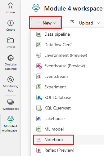
Data ingestion is the process of obtaining and importing data for immediate use or storage in a database. In Microsoft Fabric, there are several methods to ingest data, including using a data pipeline, dataflow, or notebook. Each method serves different purposes and can be chosen based on the specific requirements of the data integration scenario.
Data Pipeline
A data pipeline is a series of data processing steps. In Microsoft Fabric, you can create a data pipeline with Data Factory, which allows you to ingest raw data from various data stores into a data lakehouse. The pipeline can be automated to run on a schedule, ensuring that data is consistently and efficiently ingested into the system.
To create a data pipeline in Data Factory, you would typically:
- Navigate to the Data Factory experience within your Fabric enabled workspace.
- Create a new pipeline and define the data source, such as Blob storage.
- Specify the destination, like a Bronze table in a data lakehouse.
- Configure the data movement and transformation activities within the pipeline.
- Set up triggers to automate the pipeline execution.
For more information on creating a data pipeline, you can refer to the following tutorial: [Create a pipeline with Data Factory] https://learn.microsoft.com/en-us/fabric/data-factory/tutorial-end-to-end-introduction .
Dataflow
Dataflows are reusable data transformation processes that can be used within a data pipeline. They enable you to perform complex data transformations and manipulations before the data is loaded into the destination.
To create a dataflow in Data Factory, you would:
- Select “Dataflow Gen2” in the create menu of your workspace.
- Ingest data from a source, such as an OData service, by selecting the appropriate connector and specifying the source URL and entity.
- Add a data destination, like a lakehouse, and configure the connection settings.
- Define the transformation logic to process the ingested data.
- Publish the dataflow to make it available for use in pipelines.
For a step-by-step guide on creating a dataflow, see the tutorial: [Tutorial: Dataflows in Data Factory] https://learn.microsoft.com/en-us/fabric/data-factory/tutorial-dataflows-gen2-pipeline-activity .
Notebook
Notebooks are interactive coding environments that allow you to write, run, and debug code in a document that also contains text and visualizations. In Microsoft Fabric, you can use notebooks to orchestrate data workflows and perform data ingestion tasks.
To ingest data using a notebook, you would:
- Open the accompanying notebook for the tutorial, such as
1-ingest-data.ipynb. - Follow the instructions to import the notebook into your workspace.
- Attach a lakehouse to the notebook to ensure it has access to the necessary data storage.
- Write and execute code to ingest data from the source and load it into the lakehouse.
The accompanying notebook for the tutorial can be found here: [1-ingest-data.ipynb] https://learn.microsoft.com/en-us/fabric/data-science/tutorial-data-science-ingest-data .
Additional Resources
- For guidance on building Spark Notebook workflows using Data Factory, refer to: [Use Fabric Data Factory Data Pipelines to Orchestrate Notebook-based Workflows] https://learn.microsoft.com/en-us/fabric/data-factory/../get-started/whats-new .
- To learn about using your own Python library in the Lakehouse, visit: [Using your own library with Microsoft Fabric] https://learn.microsoft.com/en-us/fabric/data-factory/../get-started/whats-new .
- For information on logging your workload using notebooks, check out: [Logging your workload using Notebooks] https://learn.microsoft.com/en-us/fabric/data-factory/../get-started/whats-new .
By understanding and utilizing these methods, you can effectively ingest data into Microsoft Fabric, ensuring that your data is ready for analysis and further processing.
Prepare and serve data (40–45%)
Create objects in a lakehouse or warehouse
Create and Manage Shortcuts
Shortcuts in the context of data engineering are special folders that act as references to data stored in different locations, such as external Azure Data Lake storage accounts or Amazon S3. These shortcuts are particularly useful in a lakehouse architecture, allowing for seamless integration and analysis of data without the need to move or copy the data physically.
How to Create Shortcuts
- Identify the Data Source: Determine the folder in an Azure Data Lake storage or Amazon S3 account that you want to reference.
- Create a Shortcut: Use the OneLake service to create a shortcut that points to the identified folder. This involves entering connection details and credentials for the external storage account. Once created, the shortcut appears in the Lakehouse https://learn.microsoft.com/en-us/fabric/data-warehouse/get-started-lakehouse-sql-analytics-endpoint .
- SQL Analytics Endpoint: Switch to the SQL analytics endpoint within the Lakehouse. Here, you will find a SQL table that matches the name of the shortcut. This table acts as a virtual representation of the data in the external storage account https://learn.microsoft.com/en-us/fabric/data-warehouse/get-started-lakehouse-sql-analytics-endpoint .
Managing Shortcuts
- Analyzing Data: The SQL table created from the shortcut can be queried just like any other table within the SQL analytics endpoint. It allows for operations such as joining tables that reference data in different storage accounts https://learn.microsoft.com/en-us/fabric/data-warehouse/get-started-lakehouse-sql-analytics-endpoint .
- Access and Permissions: Manage access permissions to ensure that users can interact with the lakehouse data through various endpoints, including the Data Hub and the SQL analytics endpoint https://learn.microsoft.com/en-us/fabric/get-started/whats-new-archive .
- Virtualization: Shortcuts enable the virtualization of existing data into OneLake, connecting data silos without the need for data movement https://learn.microsoft.com/en-us/fabric/get-started/whats-new-archive .
Additional Information
- OneLake Shortcuts Documentation: For more detailed steps on creating and managing shortcuts within OneLake, refer to the official documentation here https://learn.microsoft.com/en-us/fabric/data-warehouse/get-started-lakehouse-sql-analytics-endpoint .
- Azure Data Lake Storage Shortcut Creation: Instructions for creating a shortcut to an Azure Data Lake storage can be found here https://learn.microsoft.com/en-us/fabric/data-warehouse/get-started-lakehouse-sql-analytics-endpoint .
- Amazon S3 Shortcut Creation: Instructions for creating a shortcut to an Amazon S3 account are available here https://learn.microsoft.com/en-us/fabric/data-warehouse/get-started-lakehouse-sql-analytics-endpoint .
- Lakehouse Sharing and Access Permission Management: Learn more about sharing a lakehouse and managing permissions here https://learn.microsoft.com/en-us/fabric/get-started/whats-new-archive .
By utilizing shortcuts, data engineers can efficiently manage and analyze data across various storage platforms, enhancing the flexibility and scalability of the lakehouse architecture.
Prepare and serve data (40–45%)
Create objects in a lakehouse or warehouse
Implementing File Partitioning for Analytics Workloads in a Lakehouse
File partitioning is a critical technique for optimizing data access in a lakehouse architecture, particularly for analytics workloads. By organizing data into partitioned datasets, queries can be executed more efficiently, as they can skip over irrelevant partitions of data. Here’s a detailed explanation of how to implement file partitioning in a lakehouse:
Understanding Data Partitioning
Data partitioning involves dividing a dataset into distinct segments,
or partitions, based on certain column values. These partitions are
typically stored in a hierarchical folder structure, such as
/year=<year>/month=<month>/day=<day>,
where year, month, and day are
the partitioning columns https://learn.microsoft.com/en-us/fabric/data-warehouse/get-started-lakehouse-sql-analytics-endpoint
. This structure allows for faster data retrieval when queries filter
data using these columns.
SQL Analytics Endpoint and Delta Lake
A SQL analytics endpoint can be used to represent partitioned Delta Lake datasets as SQL tables, enabling complex analyses on the data https://learn.microsoft.com/en-us/fabric/data-warehouse/get-started-lakehouse-sql-analytics-endpoint . Delta Lake provides versioned parquet format files that can be read and written by distributed computing systems, and the SQL analytics endpoint allows these files to be queried using SQL.
Reading and Preparing Raw Data
To create a partitioned delta table, you may start by reading raw data from the lakehouse. For instance, if the raw data is in an Excel file, you can use the pandas library to read it into a DataFrame and then add more columns for different date parts, which will be used for partitioning https://learn.microsoft.com/en-us/fabric/data-science/sales-forecasting .
import pandas as pd
df = pd.read_excel("/lakehouse/default/Files/salesforecast/raw/Superstore.xlsx")
Data Pipeline and Copy Activity
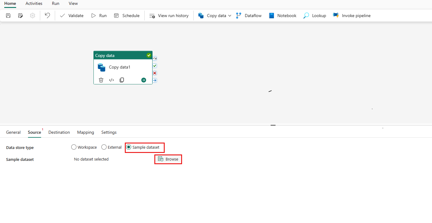
In a data pipeline, you can add a copy activity to move data from a source, such as a sample dataset, to a destination within the lakehouse. During this process, you can enable partitioning and specify the partition columns https://learn.microsoft.com/en-us/fabric/data-factory/tutorial-lakehouse-partition .
Partition Columns
When setting up the copy activity, you can choose one or multiple columns as partition columns. The partition column types can be string, integer, boolean, or datetime. The data will be partitioned by the values of these columns, and if multiple columns are used, the data is partitioned hierarchically https://learn.microsoft.com/en-us/fabric/data-factory/tutorial-lakehouse-partition .
Running the Pipeline
After configuring the partition columns, you can run the pipeline. Once the pipeline runs successfully, the data will be organized into partitions in the lakehouse, which can be verified by viewing the files in the lakehouse https://learn.microsoft.com/en-us/fabric/data-factory/tutorial-lakehouse-partition .
Benefits of Partitioning
Partitioning data in a lakehouse table offers several benefits for downstream jobs or consumption. It can significantly improve query performance by allowing the query engine to read only relevant partitions of data, reducing the amount of data scanned during query execution https://learn.microsoft.com/en-us/fabric/data-factory/tutorial-lakehouse-partition .
Additional Resources
For more information on implementing file partitioning in a lakehouse, you can refer to the following resources:
- Data partitioning in data lakes
- Tutorial on loading data to Lakehouse using partition in a Data pipeline
By following these steps and utilizing the resources provided, you can effectively implement file partitioning for analytics workloads in a lakehouse, leading to more efficient data processing and analysis.
Prepare and serve data (40–45%)
Create objects in a lakehouse or warehouse
Create Views, Functions, and Stored Procedures
Creating views, functions, and stored procedures are essential skills for managing and querying databases effectively. Below is a detailed explanation of each element:
Views
A view is a virtual table based on the result-set of an SQL statement. It contains rows and columns, just like a real table, and fields in a view are fields from one or more real tables in the database.
- Usage: Views can be used to simplify complex queries, provide a level of abstraction, or restrict access to certain data.
- Creation: You create a view by using the
CREATE VIEWstatement, followed by a SELECT query that defines the view.
Functions
Functions are routines that accept parameters, perform an action, such as a complex calculation, and return the result of that action as a value. There are two main types of functions in SQL Server:
Scalar Functions: Return a single value, based on the input value.
Table-Valued Functions: Return a table data type.
Usage: Functions can encapsulate logic that can be reused in multiple queries or stored procedures.
Creation: Functions are created using the
CREATE FUNCTIONstatement and can include complex SQL logic.
Stored Procedures
A stored procedure is a prepared SQL code that you can save and reuse over and over again. Stored procedures can take parameters so that a single procedure can be used over different data.
- Usage: They are used to encapsulate a set of operations or queries to execute on a database server. For example, operations that need to be performed on a set of data.
- Creation: Stored procedures are created with the
CREATE PROCEDUREstatement and can include complex control flow, variables, and other SQL statements.
Additional Information
For more detailed information and examples on how to create and use views, functions, and stored procedures, you can refer to the following resources:
These resources provide comprehensive guides and examples that can help you understand the syntax and usage of views, functions, and stored procedures in SQL Server. They are part of the official Microsoft documentation and are regularly updated to reflect the latest features and best practices.
Prepare and serve data (40–45%)
Create objects in a lakehouse or warehouse
Enriching Data by Adding New Columns or Tables
When working with databases, enriching data often involves adding new columns or tables to the existing schema. This process allows for the inclusion of additional information that can be used for more comprehensive analysis or reporting. Below are the steps and considerations for enriching data in this manner:
Adding New Tables or Columns
Prepare the Schema: Before adding new tables or columns, ensure that the schema is prepared to accommodate these changes. This involves planning the structure of the new tables and determining the data types and constraints for the new columns.
Manual Replication: If you are working with a synchronized database environment, you need to replicate schema changes manually to the hub and all sync members https://learn.microsoft.com/en-us/azure/azure-sql/database/sql-data-sync-sql-server-configure .
Update Sync Schema: After adding the new tables or columns to the hub and sync members, update the sync schema to include these new database objects https://learn.microsoft.com/en-us/azure/azure-sql/database/sql-data-sync-sql-server-configure .
Data Insertion: Once the schema has been updated, you can begin inserting values into the new tables and columns https://learn.microsoft.com/en-us/azure/azure-sql/database/sql-data-sync-sql-server-configure .
Considerations for Data Enrichment
Existing Data: Adding new columns will not modify or delete existing data. The new columns will be appended to the end of the schema, and the data in these new columns is typically assumed to be null unless otherwise specified https://learn.microsoft.com/azure/data-explorer/kusto/management/alter-merge-table-command .
Data Type Changes: If you are changing the data type of an existing column, the Data Sync service will continue to operate as long as the new data type is compatible with the original data type defined in the sync schema. For example, changing a column from
inttobigintwill not disrupt the Data Sync service until a value is inserted that exceeds the range of theintdata type https://learn.microsoft.com/en-us/azure/azure-sql/database/sql-data-sync-sql-server-configure .
Best Practices
Schema Evolution: When enriching data, it’s important to consider the evolution of the schema over time. Make changes in a controlled manner to avoid disrupting existing applications and services that depend on the database.
Data Integrity: Ensure that data integrity is maintained when adding new columns or tables. This includes setting appropriate constraints and considering the impact of null values.
Documentation: Keep thorough documentation of schema changes. This helps in maintaining a clear understanding of the schema’s evolution and assists in troubleshooting any issues that may arise.
For additional information on enriching data and managing schema changes, you can refer to the following resources:
By following these guidelines and considerations, you can effectively enrich your data by adding new columns or tables, thereby enhancing the capabilities of your database to meet evolving data requirements.
Prepare and serve data (40–45%)
Copy data
Choosing an Appropriate Method for Copying Data to a Lakehouse or Warehouse
When considering the transfer of data from a Fabric data source to a lakehouse or warehouse, it is essential to select a method that aligns with the volume of data, the desired level of automation, and the technical expertise available. Below are some methods and best practices to consider:
Pipeline Copy Activity
For data engineers who prefer a low-code or no-code approach, the pipeline copy activity is an excellent choice. It allows for the movement of large volumes of data, both historical and incremental, into the bronze layer of a lakehouse. This method is suitable for those who want to automate data ingestion and require minimal coding. It supports a variety of sources, including on-premises and cloud systems, and can handle petabyte-scale data transfers. The copy activity can be scheduled and is a robust choice for consolidating data into a single lakehouse https://learn.microsoft.com/en-us/fabric/data-engineering/../get-started/decision-guide-pipeline-dataflow-spark .
Automating with Data Factory
Data Factory provides a way to automate queries, data retrieval, and command execution from your warehouse. This can be particularly useful when dealing with repetitive tasks or when you need to schedule data movements. By using pipeline activities within Data Factory, you can set up a process that is both efficient and easily automated https://learn.microsoft.com/en-us/fabric/data-factory/../get-started/whats-new .
Migration Tools
For those migrating from Azure Synapse dedicated SQL pools to Microsoft Fabric, a detailed guide with a migration runbook is available. This guide provides step-by-step instructions and best practices for a smooth transition https://learn.microsoft.com/en-us/fabric/data-factory/../get-started/whats-new https://learn.microsoft.com/en-us/fabric/data-factory/../get-started/whats-new .
Data Partitioning
Efficient data partitioning is crucial for managing large datasets. Best practices and implementation guides are available to help you partition your data effectively using Fabric notebooks. This technique helps in dividing a large dataset into smaller, manageable subsets, which can improve performance and manageability https://learn.microsoft.com/en-us/fabric/data-factory/../get-started/whats-new .
SQL Analytics Endpoint Connection
For SQL users or DBAs, connecting to a SQL analytics endpoint of the Lakehouse or the Warehouse through the Tabular Data Stream (TDS) endpoint is a familiar process. This method is akin to interacting with a SQL Server endpoint and is suitable for modern web applications https://learn.microsoft.com/en-us/fabric/data-factory/../get-started/whats-new .
Additional Resources
- For more information on automating Fabric Data Warehouse queries and commands with Data Factory, you can refer to the following resource: Automate Fabric Data Warehouse Queries and Commands with Data Factory.
- To learn about migrating from Azure Synapse dedicated SQL pools, visit: Migrate from Azure Synapse dedicated SQL pools.
- For guidance on data partitioning with Microsoft Fabric, see: Efficient Data Partitioning with Microsoft Fabric: Best Practices and Implementation Guide.
- To understand how to connect to a SQL analytics endpoint, review: Microsoft Fabric - How can a SQL user or DBA connect.
By considering these methods and utilizing the available resources, you can choose the most appropriate method for copying data from a Fabric data source to a lakehouse or warehouse, ensuring efficiency and scalability in your data management strategy.
Prepare and serve data (40–45%)
Copy data
Copy Data by Using a Data Pipeline, Dataflow, or Notebook
When working with data in Azure, there are several methods to copy data depending on the use case, data size, and complexity of transformations required. Here’s a detailed explanation of each method:
Data Pipeline
A data pipeline in Azure is a series of data processing steps. One of the primary activities you can perform in a data pipeline is copying data from one location to another. The Azure Data Factory provides a visual interface to create, schedule, and manage data pipelines.
To copy data using a data pipeline: 1. Open an existing data pipeline or create a new one. 2. Use the Copy Data tool, which can be accessed from the Activities tab or by selecting Copy data on the canvas to open the Copy Assistant https://learn.microsoft.com/en-us/fabric/data-factory/tutorial-move-data-lakehouse-copy-assistant . 3. After configuring the copy activity, you can schedule the pipeline to run automatically at specified intervals.
For more information on creating your first pipeline to copy data, refer to the Quickstart: Create your first pipeline to copy data.
Dataflow
Dataflows are used for complex data transformations within Azure Data Factory or Azure Synapse Analytics. They allow you to develop data transformation logic without writing code, using a graphical interface.
To use dataflows for copying data: 1. Create a Dataflow Gen2 in Azure Data Factory. 2. Define the transformation logic within the dataflow. 3. Create a data pipeline and use the dataflow as a step within the pipeline https://learn.microsoft.com/en-us/fabric/data-factory/transform-data .
For scenarios involving small data or specific connectors, using Dataflows is recommended https://learn.microsoft.com/en-us/fabric/data-engineering/load-data-lakehouse .
Notebook
Notebooks are interactive coding environments that support languages such as Python, Scala, and SQL. They are particularly useful for exploratory data analysis and complex transformations using code.
To copy data using a notebook: 1. In the file browser, create a new subfolder where you will store your data. 2. Upload files from your local machine to the subfolder. 3. Use the Get data button to create pipelines for bulk data loads or scheduled data loads into your storage solution. 4. Utilize the Azure Blob File System (ABFS) path to access the data within the notebook for further processing https://learn.microsoft.com/en-us/fabric/onelake/create-lakehouse-onelake .
For exploring data in your lakehouse with a notebook, see Explore the data in your lakehouse with a notebook.
Additional Information
- For small file uploads from a local machine, the Local file upload method is suitable https://learn.microsoft.com/en-us/fabric/data-engineering/load-data-lakehouse .
- For large data sources, the Copy tool in pipelines is the best option https://learn.microsoft.com/en-us/fabric/data-engineering/load-data-lakehouse .
- To move data from Azure SQL DB into a lakehouse via copy assistant, refer to Move data from Azure SQL DB into Lakehouse via copy assistant.
The Azure Data Explorer connector supports organizational account authentication for both copy and Dataflow Gen2 activities https://learn.microsoft.com/en-us/fabric/data-factory/connector-azure-data-explorer . This ensures secure access to data sources when performing copy operations.
By understanding the different methods and tools available for copying data in Azure, you can choose the most appropriate approach for your specific data management needs.
Prepare and serve data (40–45%)
Copy data
Add Stored Procedures, Notebooks, and Dataflows to a Data Pipeline
When constructing a data pipeline, it is essential to integrate various activities that perform specific tasks. Stored procedures, notebooks, and dataflows are among the activities that can be added to a data pipeline to automate and streamline data processing tasks. Below is a detailed explanation of how to add each of these components to a data pipeline.
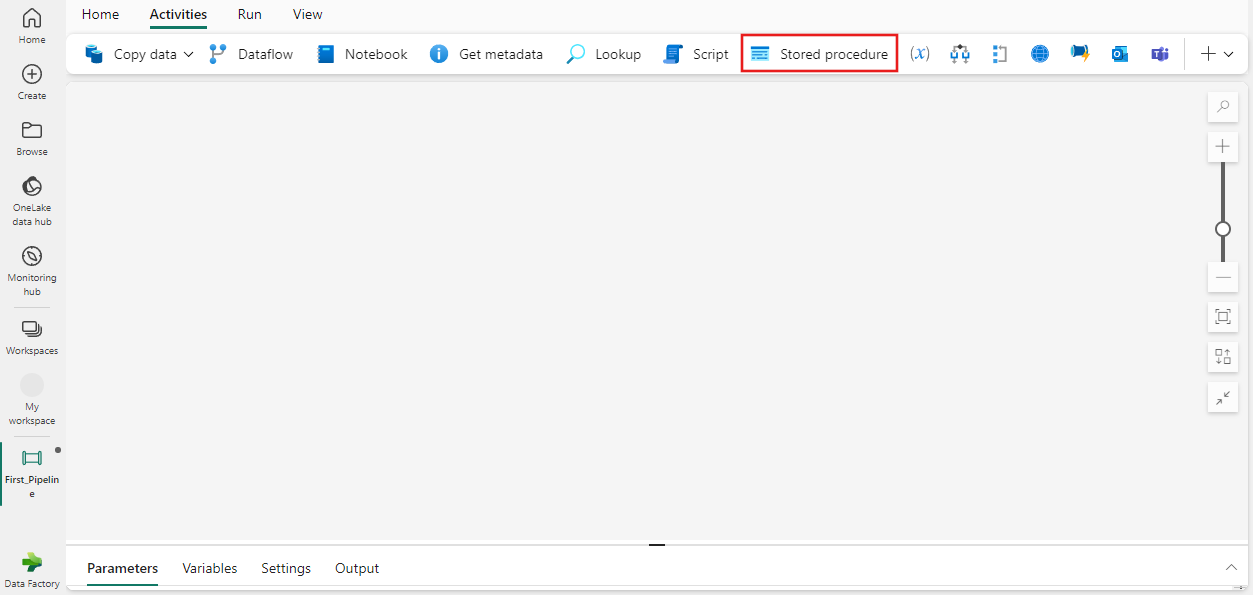
Stored Procedures
Stored procedures are precompiled collections of SQL statements that are stored under a name and processed as a unit. They can be used to encapsulate complex business logic, which can then be executed within a data pipeline.
- To add a stored procedure to your data pipeline, you must first either open an existing pipeline or create a new one.
- Within the pipeline, select the Stored Procedure activity. This activity allows you to invoke a stored procedure that is already available in your database.
- Configure the activity by specifying the linked service that connects to the database containing the stored procedure, and then select the stored procedure you wish to execute https://learn.microsoft.com/en-us/fabric/data-factory/stored-procedure-activity .
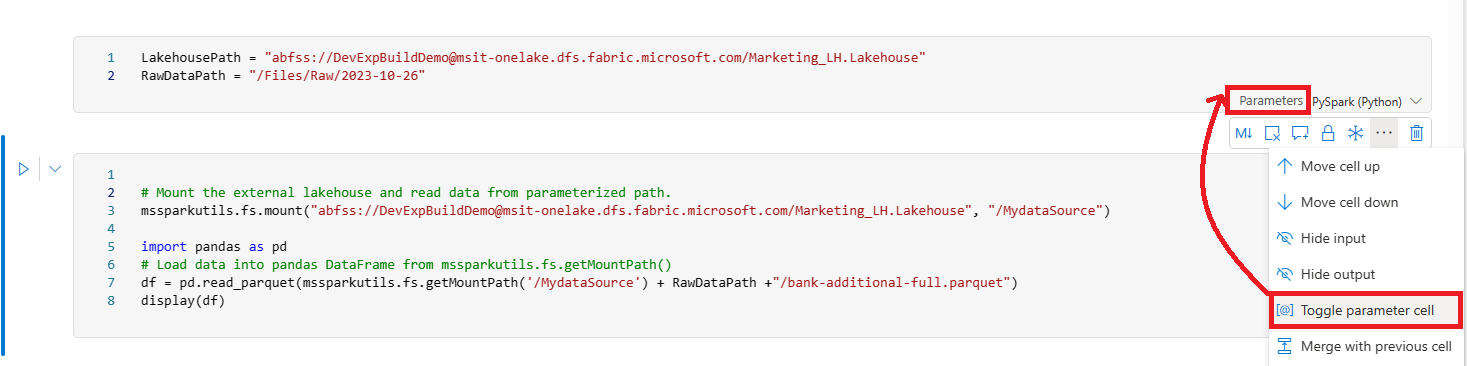
Notebooks
Notebooks are interactive coding environments that support multiple programming languages. They are commonly used for data exploration, visualization, and complex data transformations.
- Create a new notebook in your workspace or use an existing one. Notebooks can support multiple languages, but PySpark is commonly used for running Spark SQL queries.
- Add your custom code to the notebook. For example, you might include PySpark code to remove old data from a data lakehouse and prepare for new data ingestion https://learn.microsoft.com/en-us/fabric/data-factory/tutorial-setup-incremental-refresh-with-dataflows-gen2 .
- In the data pipeline, add a new Notebook activity and select the notebook you have prepared. This activity will execute the notebook as part of the pipeline run https://learn.microsoft.com/en-us/fabric/data-factory/tutorial-setup-incremental-refresh-with-dataflows-gen2 .
- To parameterize your notebook, which is useful for integrating it into a pipeline, select the ellipses (…) to access the More commands at the cell toolbar and then select Toggle parameter cell. This designates the cell as the parameters cell, which the pipeline activity will use to pass in execution-time parameters https://learn.microsoft.com/en-us/fabric/data-science/../data-engineering/author-execute-notebook .
Dataflows
Dataflows are a series of data transformations that prepare, clean, and modify data. They are defined visually in Azure Data Factory and can be executed as part of a data pipeline.
- Navigate to the workspace overview page and select Data Pipelines to create a new pipeline or modify an existing one.
- Provide a name for the data pipeline and select the Dataflow activity.
- Choose the dataflow that you have previously created from the dropdown list under Settings. This dataflow will be executed when the pipeline runs https://learn.microsoft.com/en-us/fabric/data-factory/tutorial-dataflows-gen2-pipeline-activity .
By combining these activities, you can create a robust data pipeline that automates the process of data ingestion, transformation, and loading. This pipeline can be scheduled to run on a regular basis or triggered by specific events, ensuring that your data is always up-to-date and ready for analysis.
For additional information on creating and managing data pipelines, you can refer to the following resources: - Tutorial: Set up incremental refresh with Dataflows in Azure Data Factory - Stored Procedure Activity in Azure Data Factory - Author & Execute Notebook in Azure Data Factory
Please note that the URLs provided are for reference and additional information; they should be accessed for further details on the topics discussed.
Prepare and serve data (40–45%)
Copy data
Schedule Data Pipelines
When working with data pipelines, it is often necessary to automate their execution to ensure that data processing occurs on a regular and predictable schedule. Scheduling data pipelines allows for the efficient management of data workflows without the need for manual intervention.
Steps to Schedule a Data Pipeline
Access the Pipeline Editor: Begin by navigating to the pipeline editor within your workspace.
Open the Schedule Configuration: On the Home tab of the pipeline editor window, select the Schedule option to open the schedule configuration settings https://learn.microsoft.com/en-us/fabric/data-factory/transform-data .
Set the Schedule Parameters: Configure the schedule according to your requirements. You can specify the frequency of the pipeline runs, such as daily, weekly, or monthly. Additionally, you can set the start and end dates and times for the schedule, as well as the time zone https://learn.microsoft.com/en-us/fabric/data-factory/pipeline-runs https://learn.microsoft.com/en-us/fabric/data-factory/tutorial-dataflows-gen2-pipeline-activity .
Apply the Schedule: Once you have configured the schedule settings, select Apply to activate the schedule. Your data pipeline will now run automatically according to the specified schedule https://learn.microsoft.com/en-us/fabric/data-factory/pipeline-runs https://learn.microsoft.com/en-us/fabric/data-factory/tutorial-dataflows-gen2-pipeline-activity .
Monitoring Scheduled Runs: After scheduling, you can monitor the status of your data pipeline runs by going to the Monitor Hub or by selecting the Run history tab in the data pipeline dropdown menu https://learn.microsoft.com/en-us/fabric/data-factory/tutorial-dataflows-gen2-pipeline-activity .
Additional Considerations
Frequency of Runs: The frequency of pipeline execution can be as granular as every minute or as spread out as needed, depending on the data processing requirements https://learn.microsoft.com/en-us/fabric/data-factory/tutorial-dataflows-gen2-pipeline-activity .
Timezone Settings: It is important to set the correct timezone to ensure that the pipeline runs as expected in relation to other scheduled tasks and data availability https://learn.microsoft.com/en-us/fabric/data-factory/tutorial-dataflows-gen2-pipeline-activity .
Run History and Monitoring: Keeping track of the pipeline runs is crucial for troubleshooting and ensuring data integrity. The run history provides insights into the data processed during each run.
Related Content
To learn more about creating dataflows and pipelines, as well as transforming data within these pipelines, you can refer to the documentation on creating and configuring a Dataflow Gen2 and using it in a data pipeline https://learn.microsoft.com/en-us/fabric/data-factory/transform-data .
For further details on monitoring pipeline runs and understanding the output of these runs, including the amount of data read and written, you can explore the monitoring features provided by the data pipeline tools https://learn.microsoft.com/en-us/fabric/data-factory/tutorial-move-data-lakehouse-pipeline .
Additional Resources
- For a comprehensive guide on scheduling data pipelines and other related tasks, you can visit the following URL: Schedule and Monitor Data Pipelines.
By following these steps and considerations, you can effectively schedule and manage your data pipelines, ensuring that your data processing tasks are performed reliably and efficiently.
Prepare and serve data (40–45%)
Copy data
Schedule Dataflows and Notebooks
Scheduling dataflows and notebooks is an essential aspect of automating data processing tasks within Azure services. This process allows for the execution of data transformation and analysis tasks to occur at predefined intervals, ensuring that data is consistently up-to-date and that insights are generated regularly.
Scheduling Dataflows
Dataflows are a component of Azure Data Factory, a cloud-based data integration service that allows you to create, schedule, and orchestrate your data pipelines. To schedule a dataflow:
- Open the Home tab of the pipeline editor window in Azure Data Factory.
- Select the Schedule option to configure the pipeline’s execution timing.
- Set the desired frequency and time for the pipeline to run. For example, you can schedule the pipeline to execute daily at a specific time.
By scheduling dataflows, you can automate the transformation of data and ensure that the output is stored in the appropriate data store, such as an Azure SQL database or Azure Blob Storage.
Scheduling Notebooks
Notebooks, often used for data science and batch scoring tasks, can be scheduled in various Azure services like Azure Synapse Analytics. This enables automated execution of complex data processing and machine learning tasks. To schedule a notebook:
- Utilize the Notebook scheduling capabilities within the service you are using, such as Azure Synapse Analytics.
- Notebooks can be scheduled to run as part of data pipeline activities or Spark jobs.
- In Microsoft Fabric, batch scoring notebooks can be scheduled, and the results can be seamlessly consumed from Power BI reports using Power BI Direct Lake mode.
By scheduling notebooks, data science practitioners can ensure that the latest predictions and analyses are available for stakeholders without the need for manual execution or data refreshes.
Additional Resources
For more detailed instructions and examples on scheduling dataflows and notebooks, you can refer to the following resources:
- Azure Data Factory documentation for scheduling pipelines: Schedule and run recurring tasks
- Azure Synapse Analytics documentation for scheduling notebook runs: Create, run, and manage notebooks
These resources provide step-by-step guides and best practices for effectively scheduling and automating your data processing workflows in Azure.
Remember, the ability to schedule and automate dataflows and notebooks is a powerful feature that can significantly enhance the efficiency and reliability of your data operations. It is important to familiarize yourself with the scheduling capabilities of the Azure services you are using to fully leverage the potential of cloud-based data processing.
Prepare and serve data (40–45%)
Transform data
Implementing a Data Cleansing Process
Data cleansing is a critical step in the data preparation phase, which involves identifying and correcting inaccuracies and inconsistencies in data to improve its quality. The process ensures that the data is accurate, complete, and reliable, making it suitable for analytics and decision-making. Here’s a detailed explanation of how to implement a data cleansing process:
Identify and Consolidate Data: Begin by identifying all the data sources and consolidating them into a single repository. This step is crucial for creating a unified view of the data and for the subsequent cleansing steps.
Deduplication: Check for and remove duplicate records within your data. Deduplication helps in reducing redundancy and improving the accuracy of the data.
Scrubbing and Cleansing: Scrub the data to correct misspellings, inconsistencies, and to standardize data formats. This step may involve correcting errors, filling in missing values, and standardizing text entries https://learn.microsoft.com/en-us/industry/well-architected/financial-services/operational-data-estate .
Data Enrichment: Enrich the data by adding relevant information that may be missing from the original dataset. This could involve adding additional attributes or merging with other datasets to provide a more complete picture https://learn.microsoft.com/en-us/industry/well-architected/financial-services/operational-data-estate .
Transformation: Transform the data into the required format for the target system or analysis. This may involve changing the data structure, converting data types, or applying business rules to the data https://learn.microsoft.com/en-us/industry/well-architected/financial-services/operational-data-estate .
Validation: Execute data validation scripts to ensure that the data meets the necessary quality standards before it is loaded into the target system. This step helps to avoid failures during the load process and ensures data integrity https://learn.microsoft.com/en-us/industry/well-architected/financial-services/operational-data-estate .
Logging and Monitoring: Keep track of the data cleansing process by logging activities and monitoring the success of data loads. This will help in identifying issues early and provide a way to audit the data cleansing process https://learn.microsoft.com/en-us/industry/well-architected/financial-services/operational-data-estate .
Use of Tools: Utilize ETL (Extract, Transform, Load) or ELT (Extract, Load, Transform) tools to automate the data cleansing process. These tools can help in extracting data from various sources, transforming it as per the requirements, and loading it into the target system https://learn.microsoft.com/en-us/industry/well-architected/financial-services/operational-data-estate .
For additional information and guidance on data cleansing and transformation, you can refer to the following resources:
- Overview of Microsoft Fabric, which provides a context for data science workflows: What is Microsoft Fabric? https://learn.microsoft.com/en-us/fabric/data-science/tutorial-data-science-introduction .
- Guidance on data conversion flow and the implementation phase of data projects: Data Conversion Flow and Printable PDF of Data Conversion Diagram https://learn.microsoft.com/en-us/industry/well-architected/financial-services/operational-data-estate .
- Information on data hydration for specific industries, such as financial services: Data Hydration for Microsoft Cloud for Financial Services https://learn.microsoft.com/en-us/industry/well-architected/financial-services/operational-data-estate .
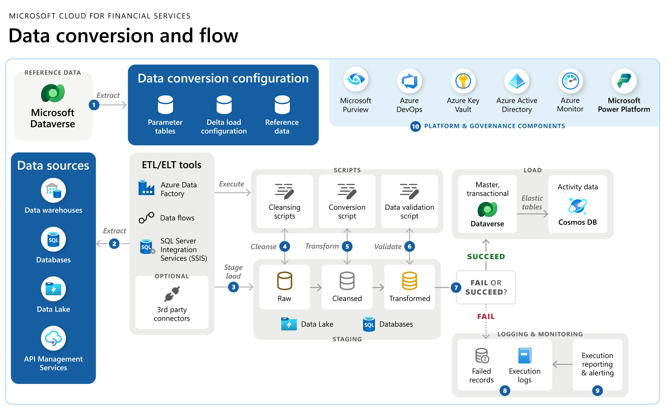
By following these steps and utilizing the provided resources, you can implement a robust data cleansing process that will prepare your data for effective analysis and reporting.
Prepare and serve data (40–45%)
Transform data
Implementing a Star Schema for a Lakehouse or Warehouse with Type 1 and Type 2 Slowly Changing Dimensions
A star schema is a data warehousing model that organizes data into fact and dimension tables, which is essential for facilitating efficient analytical processing. In a star schema, dimension tables are used to store attributes about the data, and fact tables store quantitative information. Implementing a star schema in a lakehouse or data warehouse environment involves several key considerations, especially when dealing with slowly changing dimensions (SCDs).
Type 1 Slowly Changing Dimensions
Type 1 SCDs are used when it is not necessary to keep track of historical changes in the data. When an attribute in a dimension table changes, the existing record is updated with the new information, and the old data is overwritten. This approach is simple and does not require additional storage for historical data. However, it does not provide a historical record of data changes.
Type 2 Slowly Changing Dimensions
Type 2 SCDs, on the other hand, are used to maintain a full history of data changes. When an attribute in a dimension table changes, a new record is added to the table with the updated information, and the original record is retained. Each record includes a validity period indicating when the record was active, allowing for time-travel queries to report historical data at any given point in time https://learn.microsoft.com/en-AU/azure/cosmos-db/synapse-link-time-travel .
Implementing Star Schema with SCDs
To implement a star schema that supports both Type 1 and Type 2 SCDs, follow these steps:
Design Dimension Tables: Create dimension tables that include attributes for filtering and grouping. For Type 2 SCDs, include columns to track the validity period of each record.
Design Fact Tables: Fact tables should be designed to support summarization. Ensure that fact tables load data at a consistent grain and include keys that link to the dimension tables https://learn.microsoft.com/en-us/power-bi/guidance/star-schema .
Establish Relationships: Define relationships between fact and dimension tables. The cardinality of these relationships will determine the table type (dimension or fact). Typically, a one-to-many relationship is used where the “one” side is the dimension table, and the “many” side is the fact table https://learn.microsoft.com/en-us/power-bi/guidance/star-schema .
Manage SCDs: For Type 1 changes, update the dimension table records directly. For Type 2 changes, add new records with the updated information and mark the old records as inactive or provide a validity period https://learn.microsoft.com/en-AU/azure/cosmos-db/synapse-link-time-travel .
Utilize Lakehouse Features: If implementing in a lakehouse architecture, leverage features such as ACID transactions and time-travel queries provided by systems like Delta Lake to manage SCDs effectively https://learn.microsoft.com/en-us/fabric/data-science/../data-engineering/runtime-1-2 .
Optimize for Performance: Ensure that the star schema design is optimized for query performance by minimizing joins and facilitating aggregations https://learn.microsoft.com/en-us/fabric/data-warehouse/guidelines-warehouse-performance .
For additional guidance on star schema design and slowly changing dimensions, refer to the following resources: - Star Schema in Power BI: Star Schema - Delta Lake Documentation: Delta Lake - Tables in Data Warehousing: Tables in Data Warehousing
By carefully designing and implementing a star schema that accommodates both Type 1 and Type 2 SCDs, you can create a robust data warehousing or lakehouse solution that supports comprehensive historical analysis and efficient querying.
Prepare and serve data (40–45%)
Transform data
Implementing Bridge Tables for a Lakehouse or a Warehouse
Bridge tables are a key component in data warehousing and lakehouse architectures, particularly when dealing with many-to-many relationships between tables. They are used to join entities that have a complex relationship, which cannot be represented by a simple foreign key constraint. Here’s how you can implement bridge tables in a lakehouse or warehouse environment:
Step 1: Identify Many-to-Many Relationships
First, you need to identify the many-to-many relationships within
your data model. For example, consider a scenario where you have
Products and Orders. A single order can
include multiple products, and a single product can be part of multiple
orders.
Step 2: Create the Bridge Table
Once you’ve identified a many-to-many relationship, you create a
bridge table that will hold the keys from both related tables. For
instance, you would create an OrderDetails bridge table
that contains OrderID and ProductID.
CREATE TABLE OrderDetails (
    OrderID INT NOT NULL,
    ProductID INT NOT NULL,
    Quantity INT NOT NULL
);
Step 3: Define Primary and Foreign Keys
Define the primary key for the bridge table, which is usually a composite key consisting of the foreign keys from the related tables. Also, define the foreign keys that reference the primary keys of the related tables.
ALTER TABLE OrderDetails ADD CONSTRAINT PK_OrderDetails PRIMARY KEY (OrderID, ProductID);

ALTER TABLE OrderDetails ADD CONSTRAINT FK_OrderDetails_Order FOREIGN KEY (OrderID) REFERENCES Orders (OrderID);
ALTER TABLE OrderDetails ADD CONSTRAINT FK_OrderDetails_Product FOREIGN KEY (ProductID) REFERENCES Products (ProductID);
Step 4: Populate the Bridge Table
Populate the bridge table with data that represents the relationships
between the entities. This can be done using INSERT
statements or by using INSERT...SELECT to select data from
other tables.
INSERT INTO OrderDetails (OrderID, ProductID, Quantity)
VALUES (1, 101, 2), (1, 102, 1), (2, 101, 1), (2, 103, 3);
Step 5: Querying with Bridge Tables
When querying data, you can now join the bridge table with the related tables to extract meaningful information about the many-to-many relationships.
SELECT
    Orders.OrderID,
    Products.ProductName,
    OrderDetails.Quantity
FROM
    Orders
INNER JOIN OrderDetails ON Orders.OrderID = OrderDetails.OrderID
INNER JOIN Products ON OrderDetails.ProductID = Products.ProductID;
Additional Resources
For more information on designing and querying tables in a data warehouse or lakehouse, you can refer to the following resources:
- Design tables in Warehouse in Microsoft Fabric
- Data types in Microsoft Fabric
- What is data warehousing in Microsoft Fabric?
- What is data engineering in Microsoft Fabric?
- Create a Warehouse
- Query a warehouse
By following these steps and utilizing the provided resources, you can effectively implement bridge tables in your lakehouse or warehouse to manage complex many-to-many relationships within your data model.
Prepare and serve data (40–45%)
Transform data
Denormalizing Data
Denormalization is a database optimization technique where redundant data is added to one or more tables. This can improve the performance of read operations at the expense of additional storage and potential complexity in data maintenance. In the context of data modeling, denormalization is often used to combine data from multiple normalized tables into a single table, which can simplify queries and improve data retrieval times.
Benefits of Denormalization
- Improved Query Performance: By storing related data in a single table, denormalization can reduce the need for complex joins and improve the speed of read operations https://learn.microsoft.com/en-us/power-bi/guidance/star-schema https://learn.microsoft.com/en-AU/azure/cosmos-db/nosql/modeling-data .
- Simplified Data Retrieval: Having all related data in one place can make it easier to retrieve a complete dataset with fewer queries, which can be particularly beneficial for reporting and analytics https://learn.microsoft.com/en-AU/azure/cosmos-db/nosql/modeling-data .
- Optimized for Read-heavy Workloads: Denormalized data models are often well-suited for scenarios where read operations are much more frequent than write operations, as the data is readily available in a format that’s easy to consume https://learn.microsoft.com/en-AU/azure/cosmos-db/nosql/modeling-data .
Considerations for Denormalization
- Increased Storage Requirements: Denormalization can lead to data redundancy, which may increase the storage requirements for the database.
- Data Maintenance Complexity: With redundant data, updates, inserts, and deletes can become more complex, as changes need to be propagated to all copies of the data.
- Potential for Data Inconsistency: If not managed carefully, denormalization can lead to data anomalies and inconsistencies due to the redundant nature of the data.
When to Use Denormalization
- When there are contained relationships between entities that do not frequently change https://learn.microsoft.com/en-AU/azure/cosmos-db/nosql/modeling-data .
- When there are one-to-few relationships between entities, and the data is queried together often https://learn.microsoft.com/en-AU/azure/cosmos-db/nosql/modeling-data .
- When the data model is read-heavy, and the performance of read operations is a priority.
Implementing Denormalization
In Power BI, for example, you might choose to integrate multiple related tables into a single model table to take advantage of the benefits of denormalization. This can be done by transforming and shaping the source data using tools like Power Query https://learn.microsoft.com/en-us/power-bi/guidance/star-schema .
For Azure Cosmos DB, denormalization involves embedding related subitems within a single JSON document. This approach is particularly well-suited for NoSQL databases, where schema flexibility allows for a variety of data shapes and structures https://learn.microsoft.com/en-AU/azure/cosmos-db/nosql/modeling-data https://learn.microsoft.com/en-AU/azure/cosmos-db/nosql/migrate-relational-data .
Additional Resources
For more information on data modeling and denormalization in Azure Cosmos DB, you can refer to the following resource: - Data modeling in Azure Cosmos DB
For guidance on star schema and denormalization in Power BI, the following resources may be helpful: - Star schema and its relevance to Power BI - Power Query documentation
Remember, while denormalization can offer significant benefits, it’s important to carefully consider the specific needs and usage patterns of your application to determine whether it’s the right approach for your data model.
Prepare and serve data (40–45%)
Transform data
Aggregate or De-aggregate Data
Aggregating data refers to the process of summarizing or combining data from multiple records into a single result to provide meaningful information. De-aggregating data is the reverse process, where aggregated data is broken down into its individual components. These operations are fundamental in data analysis and are used to gain insights, report on business metrics, and support decision-making.
Aggregation Techniques
Using PySpark for Aggregation: PySpark is a Python API for Spark that allows for easy data manipulation and aggregation. It is suitable for those with a programming background in Python or PySpark. PySpark can be used to join and aggregate data, which is essential for generating business insights https://learn.microsoft.com/en-us/fabric/data-engineering/tutorial-lakehouse-data-preparation .
Aggregation Pipeline in MongoDB: The aggregation pipeline is a framework provided by MongoDB for data aggregation. It consists of stages, where each stage transforms the documents as they pass through the pipeline. Common operations include filtering, grouping, sorting, transforming, and unwinding of array fields https://learn.microsoft.com/en-AU/azure/cosmos-db/mongodb/tutorial-aggregation .
- Filtering: Use
$matchto filter documents based on specific criteria. - Grouping: Use
$groupto group documents by a specified field and aggregate other fields. - Sorting: Use
$sortto order documents by one or more fields. - Transforming: Use
$projectto add, remove, or modify fields in documents. - Unwinding: Use
$unwindto deconstruct an array field from the documents to output a document for each element.
- Filtering: Use
Server-Side Aggregation in Azure Cosmos DB: Azure Cosmos DB provides
ServerSideCumulativeMetricsfor aggregating query metrics across all partitions and round trips. This feature is useful for monitoring and optimizing the performance of database queries https://learn.microsoft.com/en-AU/azure/cosmos-db/nosql/query-metrics-performance .
De-aggregation Techniques
De-aggregation is less common but can be necessary when detailed data is required from summary information. This can involve breaking down totals into individual records or distributing aggregated values across finer categories.
Spark SQL for Aggregation and De-aggregation
Spark SQL: Spark SQL is a module for structured data processing. It provides a programming abstraction called DataFrames and can also act as a distributed SQL query engine. It is a good choice for those with an SQL background transitioning to Spark https://learn.microsoft.com/en-us/fabric/data-engineering/tutorial-lakehouse-data-preparation .
- Approach #1: Use PySpark for joining and aggregating data from different dataframes, and then write the results as a delta table https://learn.microsoft.com/en-us/fabric/data-engineering/tutorial-lakehouse-data-preparation .
- Approach #2: Use Spark SQL to create a temporary view by joining tables, perform aggregation, and write the results as a delta table https://learn.microsoft.com/en-us/fabric/data-engineering/tutorial-lakehouse-data-preparation .
Both approaches are valid and can be chosen based on the user’s background and preference.
Additional Resources
- Learn about PySpark: PySpark Documentation
- Understand MongoDB’s Aggregation Pipeline: MongoDB Aggregation Pipeline
- Explore Azure Cosmos DB’s Query Metrics: Azure Cosmos DB Query Metrics
By understanding and applying these aggregation and de-aggregation techniques, one can effectively manipulate and analyze data to extract valuable insights and make informed decisions.
Prepare and serve data (40–45%)
Transform data
Merge or Join Data
Merging or joining data is a fundamental operation in data processing that combines rows from two or more tables based on a related column between them. This operation is essential for creating comprehensive datasets that provide a unified view from multiple sources.
Merge Data
Merging data typically involves combining two datasets into a single table, where the data is aligned based on common values in a column that exists in both tables. The merge operation can be performed in various ways, such as:
- Inner Merge: Combines rows from both tables that have matching values in the join columns.
- Left Outer Merge: Includes all rows from the left table and the matched rows from the right table. Unmatched rows from the right table are not included.
- Right Outer Merge: Includes all rows from the right table and the matched rows from the left table. Unmatched rows from the left table are not included.
- Full Outer Merge: Includes all rows when there is a match in either the left or right table.
In the context of Azure Data Factory, merging data can be done using the “Merge Queries” feature. This feature allows you to merge one query into another within a project, creating a new query or appending to an existing one.
Join Data
Joining data is a similar concept to merging but is often used to refer to combining data from multiple tables in a database. The join operation links data across tables based on a common field. Different types of joins include:
- Inner Join: Returns rows when there is at least one match in both tables.
- Left Join (or Left Outer Join): Returns all rows from the left table, and the matched rows from the right table. The result is NULL from the right side if there is no match.
- Right Join (or Right Outer Join): Returns all rows from the right table, and the matched rows from the left table. The result is NULL from the left side if there is no match.
- Full Join (or Full Outer Join): Returns rows when there is a match in one of the tables.
In Azure Data Explorer (Kusto), you can perform join operations by specifying the left and right tables and the conditions for matching rows. The syntax for joining tables can vary depending on whether the columns to match have the same name or different names in the tables https://learn.microsoft.com/azure/data-explorer/kusto/query/join-cross-cluster .
For more detailed guidance on joining data from multiple tables, you can refer to the tutorial provided by Azure Data Explorer https://learn.microsoft.com/azure/data-explorer/kusto/query/tutorials/use-aggregation-functions .
Additional Resources
- For more information on strategies for executing joins in Azure Data Explorer, see Strategies https://learn.microsoft.com/azure/data-explorer/kusto/query/join-cross-cluster .
- To understand how to specify the cluster or database when the data for the join resides outside the local context, refer to the cluster() and database() functions https://learn.microsoft.com/azure/data-explorer/kusto/query/join-cross-cluster .
- To learn about merge policies in Azure Data Explorer, which define how data shards get merged, visit merge policy https://learn.microsoft.com/azure/data-explorer/kusto/management/delete-database-merge-policy-command .
- For a practical example of merging queries in Power Query, including selecting join keys and kinds, see the step-by-step guide here https://learn.microsoft.com/en-us/fabric/data-factory/transform-data .
By understanding and utilizing merge and join operations, you can effectively combine data from various sources to build comprehensive datasets for analysis and reporting. These operations are crucial for data professionals who need to create relational datasets for business intelligence and data warehousing.
Prepare and serve data (40–45%)
Transform data
Identifying and Resolving Duplicate Data, Missing Data, or Null Values
When working with databases, it’s crucial to maintain data integrity and quality. Duplicate data, missing data, and null values can lead to inaccurate analyses and poor decision-making. Here’s a detailed explanation of how to identify and resolve these issues:
Duplicate Data
Duplicate data refers to records that are repeated in a dataset. This can occur due to data entry errors, data integration from multiple sources, or a lack of proper constraints in the database.
Resolution Steps: 1. Identify Duplicates: Use queries to find records with identical values in key fields. Grouping and counting records can help pinpoint duplicates. 2. Remove Duplicates: After identifying duplicates, decide on a strategy to remove them. This may involve deleting extra copies or merging records if they contain unique information. 3. Prevent Duplicates: Implement constraints like unique indexes or primary keys to prevent future duplicates. Also, establish data entry guidelines and validation rules.
Missing Data
Missing data occurs when certain fields are left blank or are not recorded. This can happen due to optional fields, errors in data collection, or during data transfer.
Resolution Steps: 1. Identify Missing
Data: Use queries to find records with NULL or
default values that indicate missing information. 2. Assess
Impact: Determine how missing data affects your analysis or
operations. Some missing values might be acceptable, while others may
need to be addressed. 3. Address Missing Data:
Depending on the situation, you might fill in missing values with
default data, use statistical methods to impute values, or reach out to
the data source for corrections.
Null Values
Null values represent the absence of data in a field. They can be intentional, indicating that data is not applicable, or unintentional, resulting from data issues.
Resolution Steps: 1. Identify Null
Values: Use queries to find fields with NULL
values. 2. Understand Context: Assess whether nulls are
appropriate for the field or if they indicate a problem. 3.
Handle Null Values: If nulls are not appropriate,
update records with correct values, or use data validation to prevent
nulls from being entered.
Additional Resources: - For more information on handling duplicate data and ensuring data uniqueness, refer to the documentation on Microsoft Sustainability Manager https://learn.microsoft.com/en-us/industry/well-architected/sustainability/sustainability-manager-data-traceability-design . - To understand how missing indexes can affect query performance and lead to missing data, review the Missing Indexes feature in SQL Server https://learn.microsoft.com/en-us/azure/azure-sql/identify-query-performance-issues . - For general guidance on query performance tuning, which can help address poorly tuned queries that might not benefit from higher compute sizes, see the section on Query Tuning and Hinting https://learn.microsoft.com/en-us/azure/azure-sql/managed-instance/performance-guidance .
By following these steps and utilizing the provided resources, you can effectively identify and resolve issues with duplicate data, missing data, or null values, ensuring the quality and reliability of your database.
Prepare and serve data (40–45%)
Transform data
Convert Data Types by Using SQL or PySpark
When working with data in SQL Server or PySpark, it’s essential to understand how to convert data types to ensure compatibility and prevent errors during data processing. Both SQL and PySpark have their own set of data types, and sometimes data needs to be converted from one type to another to perform certain operations or to integrate with other systems.
SQL Data Type Conversion
In SQL Server, data type conversion can be explicit or implicit.
Explicit conversion involves using functions like CAST or
CONVERT to change a data type deliberately. Implicit
conversion happens automatically when SQL Server determines it’s
necessary for an operation.
For example, to explicitly convert a VARCHAR data type
to an INT, you would use the following SQL syntax:
SELECT CAST(column_name AS INT) FROM table_name;
-- or
SELECT CONVERT(INT, column_name) FROM table_name;
However, not all data types can be converted directly, and attempting to do so may result in an error such as “Unhandled SQL data type” https://learn.microsoft.com/sql/machine-learning/r/r-libraries-and-data-types . It’s important to refer to the SQL Server documentation for a complete list of supported data types and conversion rules.
PySpark Data Type Conversion
PySpark, the Python API for Apache Spark, also allows for data type
conversion, which is particularly useful when working with large
datasets in distributed computing environments. PySpark uses different
functions from the pyspark.sql.functions module to perform
data type conversions.
For instance, to convert a column from StringType to
IntegerType, you can use the cast function as
follows:
from pyspark.sql.functions import col

df = df.withColumn("column_name", col("column_name").cast("int"))
In PySpark, it’s also common to use the withColumn
method to overwrite an existing column with the converted data type or
to create a new column with the converted values.
Handling Data Type Conversions Between SQL Server and R/Python
When integrating SQL Server with R or Python, data types might be implicitly converted to a compatible type. However, this conversion is not always possible, and manual intervention may be required to handle unsupported data types https://learn.microsoft.com/sql/machine-learning/r/r-libraries-and-data-types https://learn.microsoft.com/sql/machine-learning/python/python-libraries-and-data-types .
For example, when using Python integration with SQL Server Machine Learning Services, you may encounter data type conversion issues due to the limited number of data types supported by Python compared to SQL Server https://learn.microsoft.com/sql/machine-learning/python/python-libraries-and-data-types .
Additional Resources
- For more information on SQL Server data type conversions, you can refer to the official SQL Server documentation.
- To learn about PySpark data type conversions, the Apache Spark documentation provides detailed guidance.
- The PySpark API documentation is also a valuable resource for understanding the various functions available for data type conversion in PySpark.
By understanding and utilizing data type conversion functions in SQL and PySpark, you can effectively manage and transform your data to meet the requirements of different applications and systems.
Prepare and serve data (40–45%)
Transform data
Filter Data
Filtering data is a crucial aspect of managing and querying databases, as it allows users to narrow down the results to only those that are relevant to a specific criterion. Various Microsoft services and tools provide different methods to filter data effectively.
Virtual Health Data Tables
When working with virtual health data tables, it’s important to note that they support only one level of linked entity filtering. This means that when you need to filter data based on a linked entity, such as a Patient, the data must also exist on the FHIR server. An example of this would be filtering patients by their last name, such as “James”. However, there are limitations to the number of records that can be returned in a subquery, which is capped at 1,000 records. If a subquery is not selective enough and exceeds this limit, the FHIR server will return an error and no results will be produced https://learn.microsoft.com/dynamics365/industry/healthcare/use-virtual-health-data-tables .
Azure Data Lake Storage Gen1
For Azure Data Lake Storage Gen1, data can be filtered using a name range. This type of filter retrieves folders or files with names that come before or after a specified value in alphabetical order. It is a service-side filter that offers better performance compared to wildcard filters. For more detailed examples of how to use name range filters, you can refer to the Name range filter examples https://learn.microsoft.com/en-us/fabric/data-factory/connector-azure-data-lake-storage-gen1-copy-activity .
Microsoft 365 Data
When extracting data from Microsoft 365, you can use predicate expressions that filter specific rows. These expressions should match the query format of Microsoft Graph APIs. For instance, you might filter users based on their department, such as ‘Finance’. Additionally, you can select user groups from the Microsoft 365 tenant to narrow down the data retrieval to specific groups. If no groups are specified, data for the entire organization is returned. There is also the option to use a date filter, specifying a DateTime filter column to limit the time range for data extraction https://learn.microsoft.com/en-us/fabric/data-factory/connector-microsoft-365-copy-activity .
Azure Cosmos DB
In Azure Cosmos DB, you can filter metrics and charts by properties such as CollectionName, DatabaseName, PartitionKeyRangeID, and Region. By selecting these properties and their corresponding values, you can view the normalized Request Unit (RU) consumption metric for the container over a selected period. It’s important to note that for shared throughput databases, the normalized RU metric is only available at the database level and not per collection https://learn.microsoft.com/en-AU/azure/cosmos-db/monitor-normalized-request-units .
Kusto Data Ingestion
When ingesting data into a Kusto table, it’s recommended to use a single ingest client instance per hosting process, per target Kusto cluster. This is because ingest clients are reentrant and thread-safe, and creating them in large numbers is not advised. The documentation provides short code snippets demonstrating various techniques for data ingestion into Kusto tables https://learn.microsoft.com/azure/data-explorer/kusto/api/netfx/kusto-ingest-client-examples .
For additional information on filtering data in these services, you can visit the following URLs: - Virtual Health Data Tables: Filtering on a linked entity - Azure Data Lake Storage Gen1: Name range filter examples - Microsoft 365 Data: Filtering in Microsoft Graph - Azure Cosmos DB: Monitor normalized request units - Kusto Data Ingestion: Ingest data into a Kusto table
Please note that the URLs provided are for reference and additional information; they should be accessed directly for the most up-to-date guidance on filtering data within these services.
Prepare and serve data (40–45%)
Optimize performance
Identifying and Resolving Data Loading Performance Bottlenecks
When working with data processing and transformation tasks, it is crucial to identify and resolve any performance bottlenecks that may arise. Here are some strategies for addressing these issues in dataflows, notebooks, and SQL queries:
Dataflows
Understand the Data Volume: Recognize that the volume of data being processed can significantly impact performance. For low to medium data volumes, tools like Power Query and Dataflow Gen 2 offer no-code or low-code interfaces that can efficiently handle data ingestion and transformation https://learn.microsoft.com/en-us/fabric/get-started/decision-guide-pipeline-dataflow-spark .
Utilize Dataflow Gen 2: Dataflow Gen 2 is a preferred option for transforming data due to its ease of use and the ability to write results into multiple destinations. It provides over 300 data transformation options, which can be leveraged to clean and prepare data for loading into various systems https://learn.microsoft.com/en-us/fabric/get-started/decision-guide-pipeline-dataflow-spark .
Notebooks
Optimize Code: Ensure that the code written in notebooks is optimized for performance. This includes using vectorized operations, avoiding unnecessary data copies, and leveraging built-in functions that are optimized for the data processing framework in use.
Resource Management: Monitor the resources allocated to the notebook environment. Adjusting the compute resources can help alleviate bottlenecks caused by insufficient CPU or memory.
SQL Queries
Bottleneck Identification: Determine if the bottleneck is occurring while the query is in a running state or a waiting state. This distinction is crucial as it guides the approach to resolving the issue https://learn.microsoft.com/en-us/azure/azure-sql/database/identify-query-performance-issues https://learn.microsoft.com/en-us/azure/azure-sql/identify-query-performance-issues .
Use Diagnostic Tools: Employ tools like Intelligent Insights or SQL Server Dynamic Management Views (DMVs) to detect performance bottlenecks. These tools can provide insights into query performance and suggest potential resolutions https://learn.microsoft.com/en-us/azure/azure-sql/database/identify-query-performance-issues https://learn.microsoft.com/en-us/azure/azure-sql/identify-query-performance-issues .
Index Management: Azure SQL Database continuously monitors queries and suggests index creation when it identifies potential performance improvements. Index recommendations are categorized based on the estimated performance gain and are flagged as auto-created, which can be reviewed in the sys.indexes view https://learn.microsoft.com/en-us/azure/azure-sql/database/monitoring-tuning-index .
Performance Monitoring: After applying index recommendations, Azure SQL Database compares query performance against a baseline. If the new index improves performance, the recommendation is flagged as successful. Otherwise, the index is automatically reverted https://learn.microsoft.com/en-us/azure/azure-sql/database/monitoring-tuning-index .
Back-off Policy: Be aware of the back-off policy for index creation, which postpones recommendations if resource usage is high or if available storage is low. This policy ensures that database performance is not adversely affected by the creation of new indexes https://learn.microsoft.com/en-us/azure/azure-sql/database/monitoring-tuning-index .
For additional information on identifying and resolving performance bottlenecks, you can refer to the following resources:
- Azure SQL Database Performance Tuning: Identify Query Performance Issues
- Monitoring Azure SQL Database with DMVs: Monitoring with DMVs
- Azure SQL Database Index Management: sys.indexes view
By following these strategies and utilizing the provided resources, you can effectively identify and resolve data loading performance bottlenecks in various data processing environments.
Prepare and serve data (40–45%)
Optimize performance
Implement Performance Improvements in Dataflows, Notebooks, and SQL Queries
When working with dataflows, notebooks, and SQL queries, performance is a critical factor that can significantly impact the efficiency and effectiveness of data processing and analysis. Below are strategies to implement performance improvements in each area:
Dataflows
- Utilize Dataflow Gen 2: Dataflow Gen 2 offers a no-code or low-code interface for ingesting data from various sources and transforming it using over 300 data transformation options. It is designed to handle low to medium data volumes effectively https://learn.microsoft.com/en-us/fabric/get-started/decision-guide-pipeline-dataflow-spark .
- Leverage Fabric Connectors: For Dataflow Gen 2, the general availability of Fabric connectors allows seamless connection to data from Lakehouse, Warehouse, and KQL Database, which can improve the performance of data integration tasks https://learn.microsoft.com/en-us/fabric/get-started/whats-new .
- Automatic Refresh Cancellation: Dataflow Gen 2 has a mechanism that stops the refresh of a Dataflow if the results are known to have no impact, reducing unnecessary resource consumption https://learn.microsoft.com/en-us/fabric/get-started/whats-new .
- Error Message Propagation: Improved diagnostics in Dataflow Gen 2 provide meaningful error messages when a Dataflow refresh fails, aiding in quicker troubleshooting https://learn.microsoft.com/en-us/fabric/get-started/whats-new .
- Column Binding for SAP HANA Connector: Using column binding can result in significantly improved performance when connecting to SAP HANA databases https://learn.microsoft.com/en-us/fabric/get-started/whats-new .
- Staging Artifacts Hidden: In Dataflow Gen 2, staging artifacts are abstracted from the user experience, simplifying the interface and reducing clutter https://learn.microsoft.com/en-us/fabric/get-started/whats-new .
- VNet Gateways Preview: The VNet Data Gateway support for Dataflows Gen2 in Fabric helps to connect Azure data services within a VNet, enhancing security and potentially improving performance https://learn.microsoft.com/en-us/fabric/get-started/whats-new .
Notebooks
- Optimize Code: Ensure that the code within notebooks is well-optimized, using efficient algorithms and data structures.
- Parallel Processing: Take advantage of parallel processing capabilities where possible to speed up computations.
- Resource Management: Allocate appropriate resources to the notebook environment to match the workload requirements.
SQL Queries
- Query Tuning: Identify and optimize poorly tuned queries, such as those lacking a WHERE clause, missing indexes, or having outdated statistics https://learn.microsoft.com/en-us/azure/azure-sql/database/performance-guidance .
- Indexing: Implement missing indexes to speed up query execution times https://learn.microsoft.com/en-us/azure/azure-sql/database/performance-guidance .
- Statistics: Update statistics to ensure the query optimizer has accurate data distribution information, which can lead to more efficient query plans.
- Compute Size: Be aware that applications with poorly tuned queries might not benefit from a higher compute size. Instead, focus on standard query performance-tuning techniques https://learn.microsoft.com/en-us/azure/azure-sql/database/performance-guidance .
- Azure VM Performance: When running SQL Server on Azure Virtual Machines, use the same database performance tuning options as in on-premises environments, considering factors like virtual machine size and data disk configuration https://learn.microsoft.com/en-us/azure/azure-sql/virtual-machines/windows/performance-guidelines-best-practices-checklist .
For additional information and best practices, refer to the following resources: - Best practices for pg_dump and pg_restore https://learn.microsoft.com/en-AU/azure/postgresql/single-server/how-to-migrate-using-dump-and-restore . - Missing indexes https://learn.microsoft.com/en-us/azure/azure-sql/database/performance-guidance . - Query tuning and hinting https://learn.microsoft.com/en-us/azure/azure-sql/database/performance-guidance . - Medallion lake architecture https://learn.microsoft.com/en-us/fabric/get-started/whats-new . - Support for column binding for SAP HANA connector https://learn.microsoft.com/en-us/fabric/get-started/whats-new . - VNet Data Gateway support for Dataflows Gen2 in Fabric https://learn.microsoft.com/en-us/fabric/get-started/whats-new .
By implementing these performance improvements, you can ensure that your data processing workflows are optimized for speed, efficiency, and reliability.
Prepare and serve data (40–45%)
Optimize performance
Identify and Resolve Issues with Delta Table File Sizes
When working with Delta tables, it’s important to maintain optimal file sizes to ensure efficient read and write operations. Here are some strategies to identify and resolve issues with Delta table file sizes:
Identifying Issues
- Skewed Data: New data additions to Delta tables can cause data skew, leading to performance degradation https://learn.microsoft.com/en-us/fabric/data-engineering/delta-optimization-and-v-order .
- Small Files: Batch and streaming data ingestion can result in many small files, which can increase read overhead https://learn.microsoft.com/en-us/fabric/data-engineering/delta-optimization-and-v-order .
- Update/Delete Overhead: Since Parquet files are immutable, update and delete operations create new files with the changeset, which can lead to a proliferation of small files https://learn.microsoft.com/en-us/fabric/data-engineering/delta-optimization-and-v-order .
Resolving Issues
- Optimize Command: Use the
OPTIMIZEcommand to consolidate multiple small Parquet files into larger ones. This improves compression and data distribution across cluster nodes, which is beneficial for efficient read operations. It’s recommended to run optimization strategies after loading large tables https://learn.microsoft.com/en-us/fabric/data-engineering/lakehouse-table-maintenance . - V-Order: During the
OPTIMIZEcommand, you can apply V-Order, which optimizes sorting, encoding, and compression to enable fast read operations https://learn.microsoft.com/en-us/fabric/data-engineering/lakehouse-table-maintenance . For more information on V-Order, refer to Delta Lake table optimization and V-Order https://learn.microsoft.com/en-us/fabric/data-engineering/lakehouse-table-maintenance . - Vacuum Command: The
VACUUMcommand removes old files that are no longer referenced by a Delta table log. It’s important to set a retention interval that supports Delta’s time travel capabilities, with the default file retention threshold being seven days https://learn.microsoft.com/en-us/fabric/data-engineering/lakehouse-table-maintenance .
Best Practices
- Table Design: Properly designing the table’s physical structure based on ingestion frequency and expected read patterns is crucial. This can be more important than running optimization commands https://learn.microsoft.com/en-us/fabric/data-engineering/delta-optimization-and-v-order .
- Monitoring: Keep an eye on the performance and storage cost efficiency of Delta tables, and perform bin-compaction and vacuuming operations as needed https://learn.microsoft.com/en-us/fabric/data-engineering/delta-optimization-and-v-order .
Additional Resources
- For a comprehensive guide on Delta Lake table maintenance, including
the use of
OPTIMIZEandVACUUMcommands, visit Delta Lake table maintenance https://learn.microsoft.com/en-us/fabric/data-engineering/delta-optimization-and-v-order . - To understand the impact of file sizes on caching and when you might not benefit from intelligent cache, review the considerations outlined in the documentation https://learn.microsoft.com/en-us/fabric/data-science/../data-engineering/intelligent-cache .
By following these strategies and best practices, you can effectively manage Delta table file sizes, leading to improved performance and cost efficiency.
Implement and manage semantic models (20–25%)
Design and build semantic models
Choose a Storage Mode, Including Direct Lake
When designing a Power BI solution, one of the critical decisions is selecting the appropriate storage mode for your data. The storage mode determines how data is accessed and managed within Power BI. There are three primary storage modes to consider:
DirectQuery Mode: In DirectQuery mode, Power BI maintains a live connection to the data source, and queries are executed directly against the source for each user interaction. This mode does not require data to be imported into Power BI, which means that changes in the data source are immediately reflected in the Power BI reports. However, query performance depends on the speed of data retrieval from the source https://learn.microsoft.com/en-us/fabric/data-warehouse/semantic-models .
Import Mode: Import mode involves copying data into Power BI’s memory. This allows for faster query performance since the data is readily available in memory and does not need to be retrieved from the source for each query execution. However, any changes to the underlying data source are only reflected in Power BI after the next data refresh https://learn.microsoft.com/en-us/fabric/data-warehouse/semantic-models .
Direct Lake Mode: Direct Lake mode is a new capability in Power BI that allows for analyzing very large datasets. It works by loading parquet-formatted files directly from a data lake into Power BI, without querying a Warehouse or SQL analytics endpoint and without duplicating data into a Power BI semantic model. Direct Lake mode combines the benefits of DirectQuery and Import mode by providing a performant query experience and reflecting source changes as they occur. It is the default connection type for semantic models using a Warehouse or SQL analytics endpoint as a data source https://learn.microsoft.com/en-us/fabric/data-warehouse/semantic-models .
When choosing a storage mode, consider the following factors:
- Data Volume: For very large datasets, Direct Lake mode is ideal as it can handle large volumes of data efficiently https://learn.microsoft.com/en-us/fabric/data-warehouse/semantic-models .
- Data Refresh Requirements: If the data changes frequently and you need to reflect these changes quickly, DirectQuery or Direct Lake mode would be more suitable https://learn.microsoft.com/en-us/fabric/data-warehouse/semantic-models .
- Query Performance: Import mode offers better performance for datasets that fit into memory, as the data is readily available for analysis https://learn.microsoft.com/en-us/fabric/data-warehouse/semantic-models .
- Model Design: In Power BI Desktop, a mixed storage mode design results in a Composite model, where each table’s storage mode can be individually set to Import, DirectQuery, or Dual. This flexibility allows for optimizing performance and managing data volume effectively https://learn.microsoft.com/en-us/power-bi/guidance/import-modeling-data-reduction .
It is important to note that Direct Lake mode cannot be used with other storage modes in the same model. If you encounter an error related to this, ensure that all tables are set to Direct Lake mode or switch to a different storage mode that is compatible with your model design https://learn.microsoft.com/en-us/fabric/get-started/known-issues/known-issue-549-making-model-changes-semantic-model-might-not-work .
For additional information on storage modes and model design in Power BI, you can refer to the following resources:
Remember to consider the specific needs of your Power BI solution and the characteristics of your data when choosing the most appropriate storage mode.
Implement and manage semantic models (20–25%)
Design and build semantic models
Identify Use Cases for DAX Studio and Tabular Editor 2
DAX Studio and Tabular Editor 2 are powerful tools used in the context of data analysis and modeling within Microsoft’s data platform technologies. Below are the detailed use cases for each tool:
DAX Studio
DAX Studio is a tool primarily used for running DAX queries against Microsoft SQL Server Analysis Services (SSAS) tabular models, Power BI models, or Power Pivot in Excel. Its use cases include:
- Performance Tuning: Analyze and optimize the performance of DAX queries by examining query plans and server timings.
- Query Execution: Execute DAX queries to retrieve data, test measures, or calculate tables.
- Measure Development: Create and test measures before deploying them to the model.
- Data Inspection: Explore the data within the model using a tabular result of a DAX query.
- Troubleshooting: Identify and resolve issues with DAX calculations or model relationships.
For more information on DAX Studio, you can visit the official documentation: DAX Studio Documentation.
Tabular Editor 2
Tabular Editor is an advanced tool for designing Analysis Services Tabular Models in a lightweight and user-friendly environment. Its use cases include:
- Model Editing: Edit tabular model objects such as tables, columns, measures, and relationships directly outside of the Excel or Power BI environments.
- Batch Operations: Perform batch operations on metadata objects, which is particularly useful for making changes to multiple objects at once.
- Best Practice Analyzer: Use the built-in best practice analyzer to ensure the model adheres to recommended practices.
- Advanced Scripting: Automate repetitive tasks and complex modifications using the Tabular Editor’s scripting capabilities.
- Deployment: Deploy changes to different environments without affecting the existing data.
For additional information on Tabular Editor 2, refer to the following resource: Tabular Editor Documentation.
Both DAX Studio and Tabular Editor 2 are essential tools for professionals working with data models in Power BI, SSAS, or Power Pivot. They provide enhanced capabilities for query analysis, model design, and performance optimization that are not available in the standard tools provided by Microsoft.
Please note that while these tools are widely used in the industry, it is important to review the licensing terms and ensure that their use is compliant with the licensing agreements of the software being used, such as Visual Studio or SQL Server Data Tools https://learn.microsoft.com/sql/ssdt/download-sql-server-data-tools-ssdt .
Implement and manage semantic models (20–25%)
Design and build semantic models
Implementing a Star Schema for a Semantic Model
A star schema is a type of data modeling that organizes data into fact and dimension tables, which is essential for creating efficient and effective semantic models in Power BI. Implementing a star schema involves the following steps:
Identify Fact Tables: Fact tables contain the quantitative data for analysis, such as sales amounts, quantities, or other metrics. These tables typically have a large number of rows and include foreign keys that link to dimension tables https://learn.microsoft.com/en-us/fabric/data-warehouse/guidelines-warehouse-performance .
Identify Dimension Tables: Dimension tables store the descriptive attributes related to the facts. For example, a dimension table for time might include columns for the date, month, quarter, and year. Dimension tables are usually smaller and provide context for the facts https://learn.microsoft.com/en-us/fabric/data-warehouse/guidelines-warehouse-performance .
Design Relationships: Establish relationships between fact tables and dimension tables. In a star schema, each dimension table is directly linked to the fact table, creating a star-like pattern when visualized. This minimizes the number of joins required at query time, which can improve query performance https://learn.microsoft.com/en-us/fabric/data-warehouse/guidelines-warehouse-performance .
De-normalize Data: A star schema design de-normalizes the data from highly normalized Online Transaction Processing (OLTP) systems. This means combining related data into larger tables to reduce the complexity of the database structure and improve query performance https://learn.microsoft.com/en-us/fabric/data-warehouse/guidelines-warehouse-performance .
Optimize for Query Performance: By organizing data into a star schema, you reduce the number of rows read during queries and facilitate faster aggregations and grouping operations. This is because the structure is optimized for analytical processing rather than transaction processing https://learn.microsoft.com/en-us/fabric/data-warehouse/guidelines-warehouse-performance .
Utilize Data Warehousing Techniques: When modeling your data warehouse, it is recommended to use traditional Kimball methodologies and a star schema wherever possible. This involves both physical modeling (warehouse modeling) and logical modeling (semantic model modeling) https://learn.microsoft.com/en-us/fabric/data-warehouse/data-modeling-defining-relationships .
Consider Data Reduction: Implement data reduction techniques to help reduce the data loaded into Import models. This can include filtering out unnecessary columns or rows, aggregating data at a higher level, and using data compression features https://learn.microsoft.com/en-us/power-bi/guidance/overview .
For additional guidance on star schema design and its importance for Power BI, you can refer to the following resources:
- Understand star schema and the importance for Power BI: Star Schema Guidance
- Data reduction techniques for Import modeling: Data Reduction Techniques
- For more details on star schema design, consider reading “The Data Warehouse Toolkit: The Definitive Guide to Dimensional Modeling” by Ralph Kimball and others, as recommended in the literature https://learn.microsoft.com/en-us/power-bi/guidance/star-schema .
By following these steps and utilizing the provided resources, you can effectively implement a star schema for a semantic model in Power BI, leading to a data model that is optimized for both performance and usability.
Implement and manage semantic models (20–25%)
Design and build semantic models
Implementing Relationships: Bridge Tables and Many-to-Many Relationships
When designing a data model, it’s crucial to accurately represent the relationships between different entities. Two common types of relationships are one-to-many and many-to-many. To implement many-to-many relationships effectively, bridge tables, also known as factless fact tables, are often used.
Bridge Tables (Factless Fact Tables)
A bridge table is a type of factless fact table that does not contain any measure columns but only dimension keys. It is used to store observations or relationships between dimensions. For instance, a bridge table can record events such as customer logins by storing the date, time, and customer key. By counting the rows in the bridge table, you can analyze the frequency and timing of customer logins https://learn.microsoft.com/en-us/power-bi/guidance/star-schema .
Bridge tables are particularly useful for defining many-to-many dimension relationships. In a many-to-many relationship, a single entity can be associated with multiple other entities. For example, a salesperson might be assigned to multiple sales regions. The bridge table for this relationship would include two columns: one for the salesperson key and another for the region key, allowing for duplicate values in both columns https://learn.microsoft.com/en-us/power-bi/guidance/star-schema .
The use of a bridge table is recommended as a best practice for many-to-many relationships in Power BI model design. It simplifies the complexity of the relationships and makes the data model more manageable https://learn.microsoft.com/en-us/power-bi/guidance/star-schema .
Many-to-Many Relationships in Graph Databases
In addition to bridge tables, graph databases offer a way to model many-to-many relationships. Azure SQL products, for instance, provide graph database capabilities where nodes represent entities and edges represent relationships. Graph databases treat edges as first-class entities, which means they can have attributes and connect multiple nodes https://learn.microsoft.com/en-us/azure/azure-sql/multi-model-features .
Graph databases are particularly suited for:
- Modeling hierarchical data with multiple parents.
- Managing evolving applications with complex many-to-many relationships.
- Analyzing interconnected data and relationships.
- Utilizing graph-specific T-SQL search conditions, such as
SHORTEST_PATHhttps://learn.microsoft.com/en-us/azure/azure-sql/multi-model-features .
Considerations for Implementing Relationships
When implementing relationships in your data model, consider the following:
- Table Linking: Define clear and logical relationships between tables, specifying the type of relationship (one-to-many, many-to-one, or many-to-many) https://learn.microsoft.com/power-bi/create-reports/copilot-evaluate-data .
- Data Model: Choose the appropriate data model (normalized or denormalized) based on the nature of the relationships and the frequency of data changes https://learn.microsoft.com/en-AU/azure/cosmos-db/nosql/modeling-data .
- Relationship Types: Clearly specify the nature of relationships (active or inactive) and their cardinality to ensure accurate report generation https://learn.microsoft.com/power-bi/create-reports/copilot-evaluate-data .
Additional Resources
For more information on designing data models and implementing relationships, you can refer to the following resources:
- Factless Fact Table and Many-to-Many Relationships https://learn.microsoft.com/en-us/power-bi/guidance/star-schema .
- Graph Database Capabilities in Azure SQL https://learn.microsoft.com/en-us/azure/azure-sql/multi-model-features .
- Creating and Managing Relationships in Power BI Desktop https://learn.microsoft.com/en-us/power-bi/guidance/star-schema .
- Many-to-Many Relationship Guidance https://learn.microsoft.com/en-us/power-bi/guidance/star-schema .
By understanding and implementing bridge tables and many-to-many relationships, you can create a robust and scalable data model that accurately reflects the complex interconnections within your data.
Implement and manage semantic models (20–25%)
Design and build semantic models
Understanding DAX Variables and Functions for Data Modeling
Data Analysis Expressions (DAX) is a powerful language used in Power BI for creating custom calculations and measures. When working with DAX, understanding variables and functions is crucial for effective data modeling. Here’s a detailed explanation of key concepts and functions:
DAX Variables
Variables in DAX allow you to store the result of an expression as a named value. This can make your formulas easier to read and can improve performance by calculating a value once and then reusing it multiple times in your calculations. Here’s an example of how to use variables in a DAX measure:
Total Sales with Discount :=
VAR BaseSales = SUM(Sales[Amount])
VAR DiscountRate = 0.1
RETURN BaseSales - (BaseSales * DiscountRate)
In this example, BaseSales and DiscountRate
are variables that store the total sales amount and the discount rate,
respectively. The RETURN statement then uses these
variables to calculate the total sales with the discount applied.
Iterators
Iterators are DAX functions that perform row-by-row operations and
are often used with variables. Common iterators include
SUMX, AVERAGEX, MINX, and
MAXX. These functions take a table as one of their
arguments and an expression that is evaluated for each row of the table.
For example:
Average Sales per Product :=
AVERAGEX(
    Sales,
    Sales[Quantity] * Sales[UnitPrice]
)
This measure calculates the average sales per product by iterating
over each row in the Sales table and multiplying the
Quantity by the UnitPrice for each row.
Table Filtering
DAX provides functions to filter tables based on certain criteria.
The FILTER function returns a table that represents a
subset of another table, based on a provided filter expression. For
instance:
High Value Sales :=
CALCULATE(
    SUM(Sales[Amount]),
    FILTER(
        Sales,
        Sales[Amount] > 1000
    )
)
This measure sums the sales amount only for those sales that are greater than $1000.
Windowing Functions
Windowing functions in DAX allow you to create calculations that are
aware of the context in which they are executed, such as time-based
calculations. Functions like EARLIER and
EARLIEST can be used to access data from an earlier row
context. For example:
Rank Sales by Date :=
RANKX(
    ALL(Sales[SalesDate]),
    CALCULATE(SUM(Sales[Amount])),
    ,
    DESC,
    Dense
)
This measure ranks sales by date in descending order, where each sales amount is compared to all other sales amounts on different dates.
Information Functions
Information functions in DAX help you obtain metadata about the data
or the context in which a formula is being evaluated. Functions like
ISBLANK, ISERROR, ISFILTERED, and
USERNAME are commonly used. For example:
Sales for Current User :=
IF(
    ISFILTERED(User[UserName]),
    CALCULATE(
        SUM(Sales[Amount]),
        User[UserName] = USERNAME()
    ),
    SUM(Sales[Amount])
)
This measure calculates the total sales amount, but if the
User[UserName] column is filtered to the current user, it
only sums the sales for that user.
For more information on DAX and its functions, you can refer to the following resources: - DAX Basics in Power BI Desktop https://learn.microsoft.com/en-us/power-bi/guidance/star-schema - Understanding functions for parent-child hierarchies in DAX https://learn.microsoft.com/en-us/power-bi/guidance/import-modeling-data-reduction - Add calculated tables and columns to Power BI Desktop models https://learn.microsoft.com/en-us/power-bi/guidance/auto-date-time https://learn.microsoft.com/en-us/power-bi/guidance/model-date-tables
By mastering these DAX variables and functions, you can create sophisticated data models that provide deep insights and drive data-driven decision-making.
Implement and manage semantic models (20–25%)
Design and build semantic models
Implementing Calculation Groups, Dynamic Strings, and Field Parameters in Power BI
Calculation groups, dynamic strings, and field parameters are advanced features in Power BI that enable more dynamic and flexible data models and reports. Below is a detailed explanation of each feature:
Calculation Groups
Calculation groups allow you to apply common calculations across multiple measures without the need to create separate measures for each calculation. This can significantly reduce the number of measures in your model and simplify maintenance. For example, you can create a calculation group for time intelligence calculations like Month-to-Date (MTD), Quarter-to-Date (QTD), and Year-to-Date (YTD) that can be applied to any measure that calculates sales, costs, or other metrics.
To implement calculation groups in Power BI, you can use Tabular Editor, an external tool that integrates with Power BI Desktop. After creating a calculation group, you can define calculation items that represent different calculations. Each calculation item includes a DAX expression that defines the calculation logic.
For more information on calculation groups, you can refer to the official Power BI documentation on advanced data model management here https://learn.microsoft.com/power-bi/guidance/fabric-adoption-roadmap-mentoring-and-user-enablement .
Dynamic Strings
Dynamic strings in Power BI refer to the use of DAX expressions to create text values that change based on the context of the report or data model. This feature is useful for creating dynamic titles, labels, or tooltips that reflect the current filters or selections made by the user.
For instance, you can create a measure that dynamically generates a report title that includes the name of the selected category or the time period being viewed. The CONCATENATE function or the “&” operator can be used in DAX to build these dynamic strings.
Field Parameters
Field parameters are a feature in Power BI that allows report users to dynamically control which fields are used in visuals. This provides a way for users to personalize their reports by choosing the dimensions or values they want to analyze without the need for complex DAX measures or multiple visuals.
To implement field parameters, you can create a field parameter from the Modeling tab in Power BI Desktop. Once created, you can add the field parameter to a visual, and users will be able to select which fields to display from a dropdown list in the report.
For additional guidance on using field parameters, you can explore the Power BI documentation here https://learn.microsoft.com/en-us/fabric/admin/organizational-visuals .
By leveraging these advanced features, you can create more efficient and user-friendly Power BI reports and data models. Calculation groups streamline complex calculations, dynamic strings provide contextual information, and field parameters offer interactive report customization, enhancing the overall analytical capabilities of Power BI.
Implement and manage semantic models (20–25%)
Design and build semantic models
Design and Build a Large Format Dataset
When designing and building a large format dataset, it is crucial to consider several factors to ensure that the dataset is efficient, reliable, and scalable. Below are some best practices and strategies to consider:
Understand the Data Structure: The performance of your dataset will depend on the type of search queries and the structure of the data. It is essential to design your dataset with the right schema and indexing to optimize for the queries that will be run against it https://learn.microsoft.com/azure/data-explorer/kusto/query/startswith-cs-operator .
Optimize Data Operations: For large datasets, operations like dump and restore can be time-consuming. Optimizing these operations is key to maintaining efficiency. This includes understanding the impact of various factors such as network bandwidth, disk I/O, and the size of the data being moved https://learn.microsoft.com/en-AU/azure/postgresql/single-server/how-to-migrate-using-dump-and-restore .
Leverage Web-Accessible Environments: Utilize environments that provide instant access to large-scale datasets for visualization and insights. These environments should be capable of handling data synchronization and federation from various repositories and vendors, even if the data formats are incompatible https://appsource.microsoft.com/marketplace/cloudsIndustry .
Technical Staff Expertise: Ensure that the technical staff involved in the design, build, and maintenance of the infrastructure have the necessary expertise. They should be knowledgeable about handling large volumes of data and the associated systems and technologies https://learn.microsoft.com/en-us/fabric/onelake/onelake-medallion-lakehouse-architecture .
Database Connection Management: When connecting to databases, use strategies such as setting
AbortConnectto false to allow for automatic reconnection, and use a single, long-lived connection instance to avoid the overhead of establishing new connections for each request https://learn.microsoft.com/en-AU/azure/azure-cache-for-redis/cache-management-faq .Data Size Considerations: Redis, for example, works best with smaller values. Large data should be broken into multiple keys to optimize performance. Understanding the performance costs of different operations is also critical, as some commands may have a high time complexity and should be used judiciously https://learn.microsoft.com/en-AU/azure/azure-cache-for-redis/cache-management-faq .
ThreadPool Configuration: Properly configure your ThreadPool settings to prevent timeouts and ensure that your system can handle the concurrent operations without performance degradation https://learn.microsoft.com/en-AU/azure/azure-cache-for-redis/cache-management-faq .
Command Time Complexity: Be aware of the time complexity of the operations you are running. For instance, avoid using commands that have a high time complexity for large datasets, as they can significantly impact performance https://learn.microsoft.com/en-AU/azure/azure-cache-for-redis/cache-management-faq .
For additional information and detailed guidance, refer to the following resources: - Query best practices - Best practices for pg_dump and pg_restore - Connect to the cache with Redisconnection - Best practices development - Important details about ThreadPool growth - Redis command time complexity
By following these best practices, you can design and build a large format dataset that is optimized for performance, reliability, and scalability.
Implement and manage semantic models (20–25%)
Design and build semantic models
Design and Build Composite Models that Include Aggregations
When designing and building composite models in Power BI, it’s essential to understand how to effectively incorporate aggregations to optimize performance and provide a seamless analytical experience. A composite model in Power BI Desktop allows you to combine different data storage modes within a single model. You can have some tables loaded into memory (Import mode) and others queried directly from the data source (DirectQuery mode), providing flexibility and efficiency in handling large datasets https://learn.microsoft.com/en-us/power-bi/guidance/import-modeling-data-reduction .
Understanding Composite Models
Composite models enable you to determine the storage mode for each
table within your Power BI model. This means you can set the
Storage Mode property of each table to either Import,
DirectQuery, or Dual. By setting larger fact-type tables to DirectQuery,
you can reduce the overall model size and leverage the source system’s
computational power for processing large datasets. This approach is
particularly useful when you need to provide summary reporting with high
performance and also offer detailed drill-through capabilities for more
granular data https://learn.microsoft.com/en-us/power-bi/guidance/import-modeling-data-reduction
.
Implementing Aggregations
Aggregations in composite models are used to pre-calculate summaries of detailed data, which can significantly improve query performance. When a report query can be answered by the aggregation table, Power BI redirects the query to the aggregation rather than the detailed table, reducing the amount of data that needs to be processed and speeding up the response time.
To implement aggregations:
- Identify the tables and columns that are frequently queried for summaries.
- Create aggregation tables that pre-calculate these summaries and store them in the model.
- Configure the aggregation tables in Power BI Desktop to ensure that queries are appropriately redirected.
Best Practices for Composite Models with Aggregations
- Use the Mixed mode design to set larger tables to DirectQuery and smaller lookup tables to Import mode.
- Summarize large fact tables using aggregation tables to improve query performance.
- Be mindful of security and performance implications when designing composite models. It’s crucial to understand the trade-offs between data freshness, query performance, and resource utilization https://learn.microsoft.com/en-us/power-bi/guidance/import-modeling-data-reduction .
Additional Resources
For more detailed guidance on designing composite models and implementing aggregations in Power BI Desktop, refer to the following resources:
- Use composite models in Power BI Desktop
- Storage mode in Power BI Desktop
- Composite model guidance in Power BI Desktop
By following these guidelines and utilizing the resources provided, you can design and build efficient composite models that include aggregations, enhancing the analytical capabilities of your Power BI reports.
Implement and manage semantic models (20–25%)
Design and build semantic models
Implementing Dynamic Row-Level Security and Object-Level Security
Dynamic row-level security and object-level security are two important features that enhance the security of data within a database system. These features allow administrators to control access to data more granitely, ensuring that users only have access to the data they are authorized to view or manipulate.
Dynamic Row-Level Security
Dynamic row-level security (RLS) restricts access to rows in a database table based on the characteristics of the user executing a query. This could be based on group membership, execution context, or any other attribute associated with the user. RLS is particularly useful for scenarios where data access needs to be controlled at a fine-grained level, such as in multi-tenant environments where users should only see their own data.
To implement RLS, you would typically:
- Create security predicate functions that define the access logic for rows within a table.
- Apply the security predicate to the desired table as a security policy.
- Ensure that the security policy is correctly enforced whenever the table is accessed.
For more information on implementing row-level security, you can refer to the Row-Level Security documentation https://learn.microsoft.com/en-us/azure/azure-sql/database/security-overview https://learn.microsoft.com/en-us/fabric/data-warehouse/security .
Object-Level Security
Object-level security controls access to specific database objects, such as tables, views, stored procedures, and more. This type of security is used to prevent unauthorized users from accessing sensitive objects within the database.
To implement object-level security, you would:
- Use standard T-SQL constructs to grant or deny permissions on database objects to specific users or roles.
- Apply permissions at the object level to control actions such as SELECT, INSERT, UPDATE, DELETE, and EXECUTE.
- Regularly review and update permissions to ensure they align with current security requirements.
Object-level security can be combined with other security features such as column-level security, row-level security, and dynamic data masking to provide a comprehensive security strategy for your data.
For additional details on object-level security, you can explore the Object-Level Security section mentioned in the documentation https://learn.microsoft.com/en-us/fabric/data-warehouse/security .
Additional Resources
- For a comprehensive list of security features available in SQL Managed Instances, including RLS and object-level security, see the SQL Managed Instance security features article https://learn.microsoft.com/en-us/azure/azure-sql/database/authentication-azure-ad-landing .
- To understand how RLS can be applied in the context of materialized views and how to handle security policies, refer to the materialized view policies documentation https://learn.microsoft.com/azure/data-explorer/kusto/management/materialized-views/materialized-view-enable-disable .
By implementing dynamic row-level security and object-level security, administrators can ensure that data within the database is protected against unauthorized access, while still allowing users to perform their necessary tasks. These security measures are essential for maintaining data privacy and compliance with various regulatory standards.
Implement and manage semantic models (20–25%)
Design and build semantic models
Validate Row-Level Security and Object-Level Security
When preparing for a certification that covers data management and security, understanding and validating row-level security (RLS) and object-level security (OLS) is crucial. These security measures are designed to enhance data privacy and control by restricting access to data based on user roles, attributes, or other specified criteria.
Row-Level Security (RLS)
Row-level security is a feature that limits access to individual rows within a database table. This ensures that users can only view or manipulate data they are authorized to access. For instance, RLS can be used to restrict a user’s access to only those rows that are relevant to their department or to the specific data related to their company.
To validate RLS, you would typically:
Check the RLS Policy: Ensure that the RLS policy is correctly defined and associated with the relevant database tables. The policy should specify the conditions under which rows can be accessed or modified https://learn.microsoft.com/en-us/fabric/data-warehouse/security .
Test the Policy with Queries: Run queries as different users to verify that the RLS policy is enforced as expected. You can use the
set query_force_row_level_security;command to test the RLS policy without affecting other users https://learn.microsoft.com/azure/data-explorer/kusto/management/alter-materialized-view-row-level-security-policy-command .Review Materialized Views: If you are using materialized views, ensure that they have the appropriate RLS policies defined. If a materialized view is enabled without an RLS policy while the source table has one, it may lead to security issues. You can define an RLS policy over the materialized view or use the
allowMaterializedViewsWithoutRowLevelSecurityproperty to bypass this error https://learn.microsoft.com/azure/data-explorer/kusto/management/materialized-views/materialized-view-enable-disable .
For more information on RLS, you can refer to the following resources: - Row-level security policy in Azure Data Explorer https://learn.microsoft.com/azure/data-explorer/kusto/management/alter-materialized-view-row-level-security-policy-command . - Row-level security in Fabric data warehousing https://learn.microsoft.com/en-us/fabric/data-warehouse/security .
Object-Level Security (OLS)
Object-level security refers to the restrictions placed on database objects such as tables, views, stored procedures, and other entities to control which users can access them. OLS is typically managed through permissions and roles within the database management system.
To validate OLS, you should:
Review Permissions: Check the permissions assigned to different database objects and ensure they align with the intended access control policies. Permissions should be granted or denied based on the principle of least privilege.
Test Access to Objects: Similar to RLS, you can perform tests by accessing database objects as users with different roles to confirm that OLS is functioning correctly.
Audit Security Configurations: Regularly audit the security configurations for object-level permissions to prevent unauthorized access or data breaches.
While specific URLs for OLS are not provided in the retrieved documents, you can typically find information on OLS in the security documentation of the database system you are using.
By thoroughly validating RLS and OLS, you can ensure that your data management system is secure and that users have appropriate access to data and database objects. This validation is a key component of managing data privacy and security in any database environment.
Implement and manage semantic models (20–25%)
Optimize enterprise-scale semantic models
Implementing Performance Improvements in Queries and Report Visuals
When optimizing queries and report visuals, it is essential to consider several factors that can impact performance. Here are some strategies and tools that can be used to enhance the efficiency of queries and visuals in your database and reporting solutions:
Query Optimization
Understand the Data Structure: Performance is influenced by the type of search and the data structure. Familiarize yourself with the data schema and indexing to write efficient queries https://learn.microsoft.com/azure/data-explorer/kusto/query/startswith-cs-operator .
Use Query Performance Insight: For Azure SQL Database, Query Performance Insight offers intelligent analysis to identify top resource-consuming and long-running queries. This tool helps pinpoint which queries to optimize for better performance https://learn.microsoft.com/en-us/azure/azure-sql/database/query-performance-insight-use .
Analyze Resource Consumption: Look into the details of top database queries by CPU, duration, and execution count to identify potential candidates for performance improvements https://learn.microsoft.com/en-us/azure/azure-sql/database/query-performance-insight-use .
Query Details and History: Drill down into the specifics of a query to view its text and the history of resource utilization. This can provide insights into patterns of performance issues https://learn.microsoft.com/en-us/azure/azure-sql/database/query-performance-insight-use .
Performance Recommendations: Utilize the performance recommendations provided by database advisors to apply best practices and improve query efficiency https://learn.microsoft.com/en-us/azure/azure-sql/database/query-performance-insight-use .
Adjust Time Intervals: Use sliders or zoom icons in Query Performance Insight to change the observed interval, which can help in focusing on specific periods of interest https://learn.microsoft.com/en-us/azure/azure-sql/database/monitoring-tuning-index .
Enable Query Store: Ensure that Query Store is active to allow Azure SQL Database to render information in Query Performance Insight. Query Store captures query performance data over time, which is crucial for analysis https://learn.microsoft.com/en-us/azure/azure-sql/database/monitoring-tuning-index .
Report Visual Optimization
Optimize Report Designs: When reports are based on a DirectQuery semantic model, refer to the guidance provided for additional report design optimizations. This includes minimizing the number of visuals and reducing the complexity of measures https://learn.microsoft.com/en-us/power-bi/guidance/power-bi-optimization .
Monitor Performance: Identify bottlenecks by monitoring performance at design time in Power BI Desktop or on production workloads in Power BI Premium capacities. Focus on optimizing slow queries or report visuals https://learn.microsoft.com/en-us/power-bi/guidance/power-bi-optimization .
Continued Optimization: Regularly review and refine report designs and queries to maintain and improve performance. This is an ongoing process as data and business needs evolve https://learn.microsoft.com/en-us/power-bi/guidance/power-bi-optimization .
Additional Resources
- For best practices on query optimization, visit Query best practices https://learn.microsoft.com/azure/data-explorer/kusto/query/startswith-cs-operator .
- To learn more about Query Performance Insight and how to use it, check out Query Performance Insight for Azure SQL Database https://learn.microsoft.com/en-us/azure/azure-sql/database/query-performance-insight-use https://learn.microsoft.com/en-us/azure/azure-sql/database/monitoring-tuning-index .
- For guidance on optimizing Power BI report designs, refer to DirectQuery model guidance in Power BI Desktop (Optimize report designs) https://learn.microsoft.com/en-us/power-bi/guidance/power-bi-optimization .
- To understand how to monitor report performance in Power BI, visit Monitoring report performance in Power BI https://learn.microsoft.com/en-us/power-bi/guidance/power-bi-optimization .
By implementing these strategies, you can significantly improve the performance of your queries and report visuals, leading to faster insights and a better user experience.
Implement and manage semantic models (20–25%)
Optimize enterprise-scale semantic models
Improve DAX Performance by Using DAX Studio
DAX Studio is a powerful tool for writing, analyzing, and optimizing DAX expressions in Power BI, Analysis Services, and Power Pivot for Excel. Improving DAX performance involves several steps that can be facilitated by the features of DAX Studio:
Query Analysis and Optimization: DAX Studio provides a comprehensive environment to run DAX queries and view results. It allows you to measure the performance of your queries and identify bottlenecks. By analyzing the query execution, you can pinpoint inefficient measures and optimize them for better performance.
Performance Metrics: The tool offers detailed metrics and statistics about query execution, including timings and the number of storage engine queries. This information is crucial for understanding the impact of your DAX expressions on the overall performance of your model.
Server Timings and Query Plans: With DAX Studio, you can access server timings and query plans that show how the DAX engine processes your queries. This insight helps you to refine your DAX expressions to minimize the computational load and improve efficiency.
Defining and Analyzing Measures: You can define measures directly within DAX Studio and analyze their performance. This is particularly useful when you want to test different versions of a measure to determine which one is more performant.
Capturing and Analyzing Traces: DAX Studio can capture traces of what happens when a report or dashboard is interacted with. Analyzing these traces can help you understand how your DAX calculations are being used and how they perform in a real-world scenario.
Memory Usage and Data Refreshes: The tool provides insights into memory usage and data refreshes, which can help you optimize the data model for better performance. Understanding how data is loaded and stored can lead to significant improvements in DAX calculation times.
For additional information on using DAX Studio to improve DAX performance, you can refer to the following resources:
- DAX Studio Documentation
- Optimizing DAX with DAX Studio
- Using DAX Studio to Understand DAX Query Plans
By leveraging DAX Studio’s capabilities, you can ensure that your DAX expressions are as efficient as possible, leading to faster report loading times and a smoother user experience.
Implement and manage semantic models (20–25%)
Optimize enterprise-scale semantic models
Optimize a Semantic Model by Using Tabular Editor 2
When optimizing a semantic model for Power BI, Tabular Editor 2 is a powerful tool that can be used to enhance performance and manageability. Here are the steps and considerations for optimizing a semantic model using Tabular Editor 2:
Load the Semantic Model: Open Tabular Editor 2 and connect it to your Power BI dataset or Analysis Services model. This allows you to access and modify the underlying Tabular Object Model (TOM) directly.
Manage Measures and Calculations: Use Tabular Editor to create, edit, and organize measures. You can also use it to script out calculations and define calculation groups for common patterns, which can simplify the model and improve performance.
Optimize Data Model: Analyze the relationships and tables within your semantic model. Remove unnecessary columns, optimize data types, and ensure that relationships are properly defined to reduce cardinality and improve query performance.
Performance Tuning: Use Tabular Editor’s Best Practice Analyzer to identify potential performance issues and apply recommended fixes. This can include setting appropriate property values, such as
IsAvailableInMDX, or optimizing the use of row-level security.Version Control: Tabular Editor allows you to save your model’s metadata as a set of JSON files, which can be version-controlled using source control systems like Git. This helps in tracking changes and collaborating with other developers.
Deployment and Automation: With Tabular Editor, you can deploy changes directly to your Power BI service or Analysis Services instance. You can also automate deployment and other tasks using command-line scripting.
Documentation: Tabular Editor can generate documentation for your semantic model, which is essential for maintaining and understanding the model structure, especially in complex scenarios.
For additional information on using Tabular Editor 2 and optimizing semantic models, you can refer to the following resources:
- Tabular Editor documentation
- Best practices for optimizing Power BI models
- DirectQuery model guidance in Power BI Desktop
Remember to review the latest updates and features of Tabular Editor 2, as the tool is frequently updated with new capabilities that can further enhance your semantic model optimization efforts.
Implement and manage semantic models (20–25%)
Optimize enterprise-scale semantic models
Implementing Incremental Refresh
Incremental refresh is a feature that allows for efficient data importation by only bringing in new data during each refresh cycle. This process reduces the overall processing time, enabling quicker access to updated data and eliminating the need for custom solutions to import only new data https://learn.microsoft.com/en-us/industry/sustainability/sustainability-manager-import-data-incremental-refresh .
Key Concepts of Incremental Refresh
- Incremental vs. Full Refresh: Users can switch between a full refresh, which imports all data, and an incremental refresh, which imports only new data since the last refresh. This choice can be made by editing the import/connection settings https://learn.microsoft.com/en-us/industry/sustainability/sustainability-manager-import-data-incremental-refresh .
- Initial Setup: It is essential to perform a full refresh during the initial connection setup to ensure that all historical data is imported. This step also allows for the verification of correct transformations and mappings before enabling incremental refresh https://learn.microsoft.com/en-us/industry/sustainability/sustainability-manager-import-data-incremental-refresh .
- Query-Level Scheduling: Incremental refresh must be scheduled at the query level. If a data import consists of multiple queries, each one requires its own incremental refresh schedule https://learn.microsoft.com/en-us/industry/sustainability/sustainability-manager-import-data-incremental-refresh .
- Data Sources and Types: Incremental refresh supports all data sources and types, offering flexibility in scheduling across various time-bound parameters https://learn.microsoft.com/en-us/industry/sustainability/sustainability-manager-import-data-incremental-refresh .
Setting Up Incremental Refresh
- Edit Refresh Policy: Navigate to the Data imports page, select the Power Query import, and choose Edit refresh policy https://learn.microsoft.com/en-us/industry/sustainability/sustainability-manager-import-data-incremental-refresh .
- Configure Settings: In the Settings section, switch from Full refresh to Incremental refresh. This will present options to define the incremental refresh parameters https://learn.microsoft.com/en-us/industry/sustainability/sustainability-manager-import-data-incremental-refresh .
- Date/Time Column: A date or time column within the source data is required to filter for new data. Examples include Consumption start date, Consumption end date, or Transaction date https://learn.microsoft.com/en-us/industry/sustainability/sustainability-manager-import-data-incremental-refresh .
- Store and Refresh Rows: Define how far back the data needs to be stored and refreshed, specified in days, months, quarters, or years. The refresh period must not exceed the storage period https://learn.microsoft.com/en-us/industry/sustainability/sustainability-manager-import-data-incremental-refresh .
- Detect Data Changes: Opt to refresh data only when there is a change in the maximum value of a specified date or time column. This is useful when certain that no other data in the source has changed https://learn.microsoft.com/en-us/industry/sustainability/sustainability-manager-import-data-incremental-refresh .
- Complete Period Refresh: Choose to refresh data for complete periods only, ensuring consistency in the data being updated https://learn.microsoft.com/en-us/industry/sustainability/sustainability-manager-import-data-incremental-refresh .
- Save Settings: After configuring the settings, save them to schedule the incremental refresh for the selected query. Repeat the process for all necessary queries https://learn.microsoft.com/en-us/industry/sustainability/sustainability-manager-import-data-incremental-refresh .
Handling Errors and Limitations
- Error Messaging: Incremental refresh may not provide accurate error messages within the data imports due to data flow limitations. Detailed error messages can be obtained by using the data flow ID in the Power Apps portal https://learn.microsoft.com/en-us/industry/sustainability/sustainability-manager-import-data-incremental-refresh .
- Admin Credentials: The admin credentials used to connect the app to the organization’s data must remain valid over time to ensure ongoing report refreshes https://learn.microsoft.com/en-us/industry/well-architected/sustainability/emissions-impact-dashboard-deploy .
- Power BI Limitations: Access to the Power BI designer file (pbix) is not available, which restricts the use of certain tools like Performance Analyzer in Power BI Desktop https://learn.microsoft.com/en-us/industry/well-architected/sustainability/emissions-impact-dashboard-deploy .
Additional Information
For more detailed steps and visual aids on setting up incremental refresh, you can refer to the following URL: Power Apps portal.
Please note that while implementing incremental refresh, it is crucial to consider the specific requirements and limitations of the data sources and the Power BI environment to ensure successful data importation and report accuracy.
Explore and analyze data (20–25%)
Perform exploratory analytics
Implementing Descriptive and Diagnostic Analytics
Descriptive analytics involves the examination of data to understand what has happened in the past within a business or system. It typically includes the use of key performance indicators (KPIs), metrics, and data visualization tools to identify trends and patterns. Diagnostic analytics goes a step further by attempting to understand why something happened. It often involves more in-depth data analysis techniques such as drill-down, data discovery, data mining, and correlations.
Descriptive Analytics
To implement descriptive analytics, one must:
Identify Key Metrics: Determine which metrics are crucial for understanding the business or system’s performance. These could include sales figures, customer engagement levels, or operational efficiency.
Data Aggregation: Collect data from various sources and aggregate it in a way that it can be analyzed. This might involve setting up data pipelines and ensuring data quality.
Data Visualization: Use tools to create dashboards and reports that visualize the data. This helps stakeholders quickly grasp the performance and identify areas that require attention.
Regular Reporting: Establish a routine for generating and reviewing reports to keep track of performance over time.
Diagnostic Analytics
For diagnostic analytics, the following steps are typically involved:
Drill-Down Analysis: When an anomaly or a significant trend is identified in the descriptive analytics phase, use drill-down techniques to investigate the data at a more granular level to find the root cause.
Data Discovery: Employ advanced analytical techniques to uncover patterns and relationships within the data that may explain the observed phenomena.
Hypothesis Testing: Formulate hypotheses about why certain trends or patterns exist and test these using statistical methods.
Correlation Analysis: Determine the relationships between different variables to understand how they may influence each other.
Tools and Resources
To support these analytics processes, various tools and resources can be utilized:
Azure SQL Analytics: Monitor and analyze the performance of Azure SQL databases using Azure SQL Analytics, which provides advanced insights into database activity. Configure diagnostic telemetry to stream into a Log Analytics workspace for analysis https://learn.microsoft.com/en-us/azure/azure-sql/database/metrics-diagnostic-telemetry-logging-streaming-export-configure https://learn.microsoft.com/azure/azure-monitor/insights/azure-sql .
Azure Monitor: Use Azure Monitor to collect, analyze, and act on telemetry data from cloud and on-premises environments. It helps to understand how applications are performing and proactively identifies issues affecting them and the resources they depend on https://learn.microsoft.com/en-us/azure/azure-sql/database/monitor-tune-overview .
PowerShell cmdlets and Azure CLI: Configure the streaming export of diagnostic telemetry using PowerShell cmdlets or the Azure CLI for automation and scripting purposes https://learn.microsoft.com/en-us/azure/azure-sql/database/metrics-diagnostic-telemetry-logging-streaming-export-configure .
Azure Cosmos DB Diagnostic Settings: For Azure Cosmos DB, establish diagnostic settings to collect resource logs and route them to either a Log Analytics workspace or an Azure Storage account for further analysis https://learn.microsoft.com/en-AU/azure/cosmos-db/mongodb/vcore/how-to-monitor-diagnostics-logs .
By leveraging these tools and following the steps outlined above, organizations can effectively implement descriptive and diagnostic analytics to gain a better understanding of their operations and make informed decisions.
For additional information on these topics, you can refer to the following resources:
- Azure SQL Analytics documentation
- Azure Monitor documentation
- Configuring diagnostic telemetry in Azure
- Diagnostic settings for Azure Cosmos DB
Explore and analyze data (20–25%)
Perform exploratory analytics
Integrate Prescriptive and Predictive Analytics into a Visual or Report
Integrating prescriptive and predictive analytics into visuals or reports is a process that enhances decision-making by providing forward-looking insights and recommendations. Here’s a detailed explanation of how to achieve this integration:
Predictive Analytics
Predictive analytics involves using historical data, statistical algorithms, and machine learning techniques to identify the likelihood of future outcomes. This can be integrated into a visual or report by:
- Building Machine Learning Models: Utilize Azure Machine Learning or similar platforms to create predictive models based on historical data https://learn.microsoft.com/en-us/fabric/get-started/microsoft-fabric-overview .
- Experiment Tracking and Model Registry: Keep track of various experiments and manage different versions of models to ensure the best performing model is deployed https://learn.microsoft.com/en-us/fabric/get-started/microsoft-fabric-overview .
- Operationalizing Models: Deploy the trained models into production environments where they can score new data as it becomes available.
- Visualization: Incorporate the predictions from the models into reports or dashboards using tools like Power BI, displaying predicted values alongside actual data for comparison.
Prescriptive Analytics
Prescriptive analytics goes a step further by not only predicting outcomes but also suggesting actions to benefit from the predictions. This can be integrated into a visual or report by:
- Maintenance Recommendations: Use prescriptive analytics to recommend maintenance activities that prevent costly disruptions, optimizing operations.
- Advanced Analytics Concepts: Introduce concepts like predictive and prescriptive analytics into reports, especially if they are new to the user community. This could involve explaining the statistical models or algorithms used in layman’s terms https://learn.microsoft.com/power-bi/guidance/fabric-adoption-roadmap-change-management .
- Interactive Data: Enable users to interact with the data and models directly in the report, such as drilling down into specific predictions or altering input variables to see how the recommendations change https://learn.microsoft.com/power-bi/guidance/fabric-adoption-roadmap-change-management .
Best Practices for Integration
- Incremental Changes: Implement changes gradually to allow users to adapt to new analytics concepts and the enhanced reports https://learn.microsoft.com/power-bi/guidance/fabric-adoption-roadmap-change-management .
- User Education: Educate the user community on the value and interpretation of predictive and prescriptive insights to ensure they are leveraged effectively https://learn.microsoft.com/power-bi/guidance/fabric-adoption-roadmap-change-management .
- Feedback Loop: Establish a feedback mechanism to continuously improve the analytics models and the reports based on user interaction and changing business needs https://learn.microsoft.com/power-bi/guidance/fabric-adoption-roadmap-change-management .
For additional information on integrating analytics into your solutions, you can refer to the following resources: - Shared Semantic Model - Personal Usage Scenarios - Azure Machine Learning - Azure SQL Analytics
By following these guidelines, you can effectively integrate prescriptive and predictive analytics into your visuals and reports, providing actionable insights that drive business value.
Explore and analyze data (20–25%)
Perform exploratory analytics
Profile Data in Azure SQL Monitoring and Microsoft Sustainability Manager
When working with Azure SQL and Microsoft Sustainability Manager, understanding and managing profile data is crucial for effective monitoring and data analysis. Here’s a detailed explanation of profile data in these contexts:
Azure SQL Monitoring Profiles
In Azure SQL, a monitoring profile is a set of configurations that determine what data is collected from SQL systems and how it is stored. These profiles are essential for administrators to monitor the health and performance of their SQL databases and managed instances.
Key Components of a Monitoring Profile:
- Name: A unique identifier for the profile, which cannot be changed after creation.
- Location: The Azure region where the profile is stored. It should match the location of the Log Analytics workspace.
- Log Analytics Workspace: The destination for the monitoring data collected by the profile.
- Collection Settings: Defines the frequency and type of SQL monitoring data to be collected.
To create a new monitoring profile, navigate to the Insights section of the Azure Monitor menu in the Azure portal and select SQL (preview). From there, you can select Create new profile and specify the settings for your SQL systems, such as Azure SQL Database, Azure SQL Managed Instance, or SQL Server running on virtual machines https://learn.microsoft.com/en-us/azure/azure-sql/database/sql-insights-enable .
Microsoft Sustainability Manager Calculation Profiles
In Microsoft Sustainability Manager, a calculation profile is a configuration that determines how data is applied to calculations for generating carbon emissions or water usage data. These profiles are vital for narrowing down the data used in analyses, reports, and scorecards.
Steps to Create a Calculation Profile:
- Navigate to Calculations on the left navigation pane and select Calculation profiles.
- Click on New Calculation profile and enter the required values, such as the profile name, emissions source, and activity data to include in the calculation.
- Choose the appropriate calculation model and verify the results before letting it run https://learn.microsoft.com/en-us/industry/sustainability/data-model-extend .
Calculation profiles allow for precise control over the data and frequency of calculations, ensuring that only relevant data is included in environmental impact assessments.
Additional Resources
For more information on creating and managing monitoring profiles in Azure SQL, you can refer to the data collection rule resource overview.
For guidance on setting up calculation profiles in Microsoft Sustainability Manager, the data model extension documentation provides a visual aid and additional details.
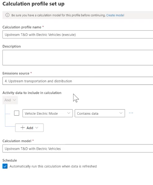
By understanding and effectively utilizing profile data in Azure SQL and Microsoft Sustainability Manager, organizations can enhance their monitoring capabilities and make informed decisions based on accurate environmental data.
Explore and analyze data (20–25%)
Query data by using SQL
Querying a Lakehouse in Fabric Using SQL Queries or the Visual Query Editor
When working with a lakehouse in Fabric, you have the flexibility to query data using SQL queries or the visual query editor. Here’s a detailed explanation of how to perform these actions:
Using SQL Queries
Cross-Database Queries: Within the same Fabric workspace, you can write cross-database queries to databases in the current active workspace. This can be done by joining tables or views to run cross-warehouse queries https://learn.microsoft.com/en-us/fabric/data-warehouse/query-warehouse .
Adding SQL Analytics Endpoint or Warehouse: To reference databases when writing a SQL query, you first need to add a SQL analytics endpoint or Warehouse from your current active workspace to the object Explorer using the “+ Warehouses” action https://learn.microsoft.com/en-us/fabric/data-warehouse/query-warehouse .
Three-Part Naming: You can reference tables from added databases using three-part naming. For example, to refer to
ContosoSalesTablein the added databaseContosoLakehouse, you would use the following syntax:SELECT * FROM ContosoLakehouse.dbo.ContosoSalesTable AS Contoso INNER JOIN Affiliation ON Affiliation.AffiliationId = Contoso.RecordTypeID;This allows you to join multiple databases using their three-part names https://learn.microsoft.com/en-us/fabric/data-warehouse/query-warehouse .
Aliases for Efficiency: For more efficient and longer queries, you can use aliases to simplify the query and make it more readable https://learn.microsoft.com/en-us/fabric/data-warehouse/query-warehouse .
Inserting Data Across Databases: Using the three-part naming convention, you can also insert data from one database to another. This is useful for data migration or consolidation tasks https://learn.microsoft.com/en-us/fabric/data-warehouse/query-warehouse .
Using the Visual Query Editor
Drag and Drop Interface: The visual query editor provides a user-friendly interface where you can drag and drop tables from added databases to create a cross-database query. This method is particularly useful for those who prefer a more visual approach to query construction https://learn.microsoft.com/en-us/fabric/data-warehouse/query-warehouse .
Creating Lakehouse: When you create a lakehouse in Fabric, a Warehouse is automatically created along with a SQL analytics endpoint. This endpoint allows you to query data in the Lakehouse using T-SQL language https://learn.microsoft.com/en-us/fabric/data-warehouse/get-started-lakehouse-sql-analytics-endpoint .
SQL Analytics Endpoint: The SQL analytics endpoint is automatically generated for every Lakehouse and exposes Delta tables as SQL tables that can be queried using T-SQL. There’s no need for users to create a SQL analytics endpoint manually https://learn.microsoft.com/en-us/fabric/data-warehouse/get-started-lakehouse-sql-analytics-endpoint .
Additional Considerations
- Session Context: In the SQL query editor, each query run opens a separate session and closes it at the end of execution. This means that session context is not maintained across multiple query runs https://learn.microsoft.com/en-us/fabric/data-warehouse/sql-query-editor .
- Supported Statements: You can run DDL, DML, and DCL statements, but there are limitations for TCL statements. For example, transactions must be executed as a single batch request to retain the session context https://learn.microsoft.com/en-us/fabric/data-warehouse/sql-query-editor .
- Visualize Results: The Visualize Results feature currently does not support SQL queries with an ORDER BY clause https://learn.microsoft.com/en-us/fabric/data-warehouse/sql-query-editor .
Related Content
- For more information on how to use the SQL query editor and the visual query editor, you can refer to the following resources:
By understanding these methods and considerations, you can effectively query a lakehouse in Fabric using the method that best suits your needs and preferences.
Explore and analyze data (20–25%)
Query data by using SQL
Querying a Warehouse in Fabric Using SQL Queries or the Visual Query Editor
When working with a warehouse in Microsoft Fabric, you have the flexibility to query your data using either SQL queries or the visual query editor. Both methods offer efficient ways to interact with your data, and the choice between them depends on your preference for a code-based or a no-code experience.
Using SQL Queries
SQL queries are a powerful way to interact with your data. You can write and execute Transact-SQL (T-SQL) queries directly from the Microsoft Fabric portal using the SQL query editor. This method is suitable for those who are comfortable with writing SQL code and require the precision and control that T-SQL offers.
SQL Query Editor: The SQL query editor in the Microsoft Fabric portal allows you to write T-SQL queries. It supports features like IntelliSense, code completion, syntax highlighting, client-side parsing, and validation. You can run Data Definition Language (DDL), Data Manipulation Language (DML), and Data Control Language (DCL) statements within this editor https://learn.microsoft.com/en-us/fabric/data-warehouse/sql-query-editor .
Cross-Database Queries: You can also write cross-database queries using three-part naming to reference
database.schema.table, similar to SQL Server. This is particularly useful when joining data from different sources within your warehouse https://learn.microsoft.com/en-us/fabric/data-warehouse/tutorial-sql-cross-warehouse-query-editor .
Using the Visual Query Editor
For those who prefer a no-code experience, the visual query editor provides a user-friendly interface to create queries without writing code. This can be especially helpful for users who are not familiar with SQL or who want to build queries quickly and visually.
No-Code Experience: The visual query editor in the Microsoft Fabric portal offers a no-code experience, allowing you to create queries by selecting options and fields from a graphical interface https://learn.microsoft.com/en-us/fabric/data-warehouse/visual-query-editor .
Data Preview: You can quickly view data in the Data preview to ensure that your queries are returning the expected results https://learn.microsoft.com/en-us/fabric/data-warehouse/visual-query-editor .
Additional Resources
To enhance your understanding and capabilities when querying a warehouse in Microsoft Fabric, you can refer to the following resources:
For more information on how to use the visual query editor, visit the Visual Query Editor documentation https://learn.microsoft.com/en-us/fabric/data-warehouse/visual-query-editor .
To learn about querying the data in your warehouse with multiple tools, including using a SQL connection string, refer to the Query Warehouse documentation https://learn.microsoft.com/en-us/fabric/data-warehouse/visual-query-editor .
For a tutorial on creating and executing T-SQL queries with the SQL query editor, see the SQL Query Editor tutorial https://learn.microsoft.com/en-us/fabric/data-warehouse/tutorial-sql-cross-warehouse-query-editor .
To get started with connecting to your Warehouse in Microsoft Fabric, check out the Connectivity documentation https://learn.microsoft.com/en-us/fabric/data-warehouse/create-table .
By utilizing these resources, you can effectively query your warehouse in Microsoft Fabric using the method that best suits your needs and expertise.
Explore and analyze data (20–25%)
Query data by using SQL
Connect to and Query Datasets Using the XMLA Endpoint
The XMLA endpoint is a feature in Power BI that allows for connectivity with Microsoft and third-party tools, enabling various operations such as querying and managing datasets within Power BI semantic models. To utilize the XMLA endpoint for connecting to and querying datasets, follow these steps:
- Scripting the Semantic Model:
- Use SQL Server Management Studio (SSMS) to script out the default Power BI semantic model from the XMLA endpoint. This can be done by viewing the Tabular Model Scripting Language (TMSL) schema of the semantic model.
- To connect, you will need the semantic model’s connection string,
which typically follows the format
powerbi://api.powerbi.com/v1.0/myorg/username. This connection string can be found in the Power BI Service under Settings > Server settings. - Once connected, you can generate an XMLA script of the semantic model using the Script context menu action in SSMS’s Object Explorer. For additional guidance, refer to the documentation on Dataset connectivity with the XMLA endpoint.
- Monitoring with SQL Server Profiler:
- SQL Server Profiler, which is included with SSMS, allows you to trace and debug events on the semantic model by connecting to the XMLA endpoint.
- Ensure you have SQL Server Profiler version 18.9 or higher, and specify the semantic model as the initial catalog when establishing the connection.
- For more information on using SQL Server Profiler with Analysis Services and Power BI, see the SQL Server Profiler for Analysis Services documentation.
- Editing Data Models in Power BI Service:
- Users can edit data models in the Power BI service through the tenant settings. However, this does not apply to DirectLake datasets or editing a dataset through an API or XMLA endpoint.
- To enable data model editing in the admin portal, consult the Enabling data model editing in the admin portal guide.
- Configuring XMLA Endpoint Settings:
- In the Power BI admin portal, you can configure the XMLA endpoint settings to control access levels, such as turning off the endpoint or setting it to read-only or read-write modes.
- For a comprehensive understanding of these settings, review the XMLA endpoints documentation.
- Using Excel with Power BI Semantic Models:
- When enabled, organization users can leverage Excel to view and interact with on-premises Power BI semantic models, which also involves connecting to XMLA endpoints.
- For instructions on creating Excel workbooks with refreshable Power BI data, refer to the guide on Create Excel workbooks with refreshable Power BI data.
By following these steps and utilizing the provided resources, you can effectively connect to and query datasets using the XMLA endpoint in Power BI.
Explore and analyze data (20–25%)
Query data by using SQL
Connect to and Query Datasets Using the XMLA Endpoint
The XMLA endpoint is a feature in Power BI that allows for connectivity with Microsoft and third-party tools, enabling various operations such as querying and managing datasets within Power BI semantic models. To utilize the XMLA endpoint for connecting to and querying datasets, follow these steps:
- Scripting the Semantic Model:
- Use SQL Server Management Studio (SSMS) to script out the default Power BI semantic model from the XMLA endpoint.
- Obtain the Tabular Model Scripting Language (TMSL) schema of the semantic model by scripting it out via the Object Explorer in SSMS.
- Connect using the semantic model’s connection string, which
typically follows the format
powerbi://api.powerbi.com/v1.0/myorg/username. - The connection string can be found in the Power BI Settings under Server settings.
- Generate an XMLA script of the semantic model using SSMS’s Script context menu action https://learn.microsoft.com/en-us/fabric/data-warehouse/semantic-models .
- Monitoring and Analyzing Activity:
- SQL Server Profiler can be used to monitor and analyze activity on the semantic model by connecting to the XMLA endpoint.
- Ensure that SQL Server Profiler version 18.9 or higher is installed, which comes with SSMS.
- When connecting, specify the semantic model as the initial catalog https://learn.microsoft.com/en-us/fabric/data-warehouse/semantic-models .
- Editing Data Models:
- Users can edit data models in the Power BI service (preview) tenant settings, but this does not apply to DirectLake datasets or editing a dataset through an API or XMLA endpoint https://learn.microsoft.com/en-us/fabric/admin/service-admin-portal-data-model .
- XMLA Endpoint Settings:
- Configure XMLA endpoint settings in the Power BI service to determine if they are turned off, or set to read-only or read-write modes, especially in the Power BI Premium Per User (PPU) capacity https://learn.microsoft.com/en-us/fabric/admin/service-admin-portal-premium-per-user .
- Using Excel with Semantic Models:
- When enabled, users can use Excel to view and interact with on-premises Power BI semantic models, which also involves connecting to XMLA endpoints https://learn.microsoft.com/en-us/fabric/admin/service-admin-portal-integration .
For additional information on these topics, you can refer to the following resources: - Dataset connectivity with the XMLA endpoint https://learn.microsoft.com/en-us/fabric/data-warehouse/semantic-models . - SQL Server Profiler for Analysis Services https://learn.microsoft.com/en-us/fabric/data-warehouse/semantic-models . - Enabling data model editing in the admin portal https://learn.microsoft.com/en-us/fabric/admin/service-admin-portal-data-model . - XMLA endpoints in Power BI https://learn.microsoft.com/en-us/fabric/admin/service-admin-portal-premium-per-user . - Create Excel workbooks with refreshable Power BI data https://learn.microsoft.com/en-us/fabric/admin/service-admin-portal-integration .
By following these guidelines and utilizing the provided resources, users can effectively connect to and query datasets using the XMLA endpoint in Power BI.