DP-602 Study Guide

Prepare and serve data
Create objects in a lakehouse or warehouse
Ingesting Data Using a Data Pipeline, Dataflow, or Notebook
Data ingestion is a critical step in the data processing lifecycle, where data is imported, transferred, loaded, and processed from various sources into a system where it can be stored, analyzed, and utilized. There are several methods to perform data ingestion in Azure, including using a data pipeline, dataflow, or notebook. Below is a detailed explanation of each method:
Data Pipeline
A data pipeline is a series of data processing steps. In Azure Data Factory, a data pipeline can be created to automate the movement and transformation of data. Here’s how you can create and use a data pipeline:
- Navigate to your workspace and select the +New button, then choose Data pipeline https://learn.microsoft.com/en-us/fabric/data-warehouse/ingest-data-pipelines .
- Provide a name for your new pipeline and select Create https://learn.microsoft.com/en-us/fabric/data-warehouse/ingest-data-pipelines .
- In the pipeline canvas, you have options like Add a pipeline activity, Copy data, and Choose a task to start. For data ingestion, you can use the Copy data option https://learn.microsoft.com/en-us/fabric/data-warehouse/ingest-data-pipelines .
- The Copy data assistant helps you select a data source and destination, configure data load options, and create a new pipeline activity with a Copy Data task https://learn.microsoft.com/en-us/fabric/data-warehouse/ingest-data-pipelines .
- After configuring the source and destination, you can run the pipeline immediately or schedule it for later execution https://learn.microsoft.com/en-us/fabric/data-warehouse/ingest-data-pipelines .
For more information on creating data pipelines, you can refer to the following URL: Ingesting data into the Warehouse.
Dataflow
A dataflow is a reusable data transformation that can be used in a pipeline. It allows for complex data transformations and manipulations. Here’s how to create a dataflow:
- Switch to the Data Factory experience https://learn.microsoft.com/en-us/fabric/data-factory/tutorial-dataflows-gen2-pipeline-activity .
- Go to your workspace and select Dataflow Gen2 in the create menu https://learn.microsoft.com/en-us/fabric/data-factory/tutorial-dataflows-gen2-pipeline-activity .
- Ingest data from your source, such as an OData source, by selecting Get data and then More https://learn.microsoft.com/en-us/fabric/data-factory/tutorial-dataflows-gen2-pipeline-activity .
- Choose the data source, enter the URL, and select the entity you want to ingest https://learn.microsoft.com/en-us/fabric/data-factory/tutorial-dataflows-gen2-pipeline-activity .
- Set up the lakehouse destination by selecting Add data destination and then Lakehouse https://learn.microsoft.com/en-us/fabric/data-factory/tutorial-dataflows-gen2-pipeline-activity .
- Configure the connection, confirm the table name, and select the update method https://learn.microsoft.com/en-us/fabric/data-factory/tutorial-dataflows-gen2-pipeline-activity .
- Publish the dataflow to make it available for use in data pipelines https://learn.microsoft.com/en-us/fabric/data-factory/tutorial-dataflows-gen2-pipeline-activity .
For additional details on creating dataflows, visit: Tutorial: Create a dataflow.
Notebook
Notebooks in Azure Databricks or Azure Synapse Analytics provide an interactive environment for data engineering, data exploration, and machine learning. To ingest data using a notebook:
- Import the notebook to your workspace following the instructions provided in the tutorial https://learn.microsoft.com/en-us/fabric/data-science/tutorial-data-science-ingest-data .
- Attach a lakehouse to the notebook before running any code https://learn.microsoft.com/en-us/fabric/data-science/tutorial-data-science-ingest-data .
- Use the notebook to write and execute code that ingests data from various sources into your data lake or data warehouse https://learn.microsoft.com/en-us/fabric/data-science/tutorial-data-science-ingest-data .
The accompanying notebook for data ingestion tutorials can be found here: 1-ingest-data.ipynb.
For guidance on using Azure Databricks interface to explore raw source data, see: Explore the source data for a data pipeline.
By utilizing these methods, you can effectively ingest data into your Azure environment, setting the stage for further data processing and analysis.
Prepare and serve data
Create objects in a lakehouse or warehouse
Create and Manage Shortcuts
Shortcuts in the context of data engineering are references to folders in external storage accounts that are managed by data processing engines like Synapse Spark or Azure Databricks. These shortcuts act as virtual warehouses and can be leveraged for downstream analytics or queried directly. Here’s a detailed explanation of how to create and manage these shortcuts:
- Creating a Shortcut:
- To create a shortcut, you need to reference a folder in an Azure Data Lake storage or an Amazon S3 account. This involves entering connection details and credentials, after which the shortcut appears in the Lakehouse https://learn.microsoft.com/en-us/fabric/data-warehouse/get-started-lakehouse-sql-analytics-endpoint .
- The shortcut creation process is straightforward and can be initiated by following the guidelines provided in the official documentation for creating an Azure Data Lake storage shortcut or an Amazon S3 shortcut https://learn.microsoft.com/en-us/fabric/data-warehouse/get-started-lakehouse-sql-analytics-endpoint .
- Managing Shortcuts:
- Once a shortcut is created, it can be managed through the SQL analytics endpoint of the Lakehouse. A SQL table with a name matching the shortcut name will be available, which references the folder in the external storage account https://learn.microsoft.com/en-us/fabric/data-warehouse/get-started-lakehouse-sql-analytics-endpoint .
- This SQL table can be queried like any other table within the SQL analytics endpoint, allowing for operations such as joining tables that reference data in different storage accounts https://learn.microsoft.com/en-us/fabric/data-warehouse/get-started-lakehouse-sql-analytics-endpoint .
- It is important to note that there might be a delay in the SQL table showing up in the SQL analytics endpoint, so a few minutes of wait time may be required https://learn.microsoft.com/en-us/fabric/data-warehouse/get-started-lakehouse-sql-analytics-endpoint .
- Using Shortcuts for Data Analysis:
- Shortcuts can be analyzed from a SQL analytics endpoint, and a SQL table is created for the referenced data. This enables the exposure of data in externally managed data lakes and facilitates analytics on them https://learn.microsoft.com/en-us/fabric/data-warehouse/get-started-lakehouse-sql-analytics-endpoint .
- The shortcut essentially acts as a virtual warehouse that can be used for additional downstream analytics requirements or queried directly https://learn.microsoft.com/en-us/fabric/data-warehouse/get-started-lakehouse-sql-analytics-endpoint .
- Benefits of Shortcuts:
- Shortcuts provide a means to connect data silos without the need to move or copy data, thus simplifying the data virtualization process https://learn.microsoft.com/en-us/fabric/get-started/whats-new-archive .
- They enable the use of historical data in OneLake without the need for data copying, which is particularly useful for managing large datasets and reducing the time and resources required for data migration https://learn.microsoft.com/en-us/fabric/data-engineering/migrate-synapse-data-pipelines .
For additional information on creating and managing shortcuts, you can refer to the following resources: - Create a shortcut in Azure Data Lake storage - Create a shortcut in Amazon S3 account - Virtualize your existing data into OneLake with shortcuts
By understanding and utilizing shortcuts, data engineers can efficiently manage data across different storage solutions, enabling seamless analytics and data processing within a unified architecture.
Prepare and serve data
Create objects in a lakehouse or warehouse
Implementing File Partitioning for Analytics Workloads in a Lakehouse
File partitioning is a critical technique for optimizing data access
in a lakehouse architecture. By organizing data into hierarchical folder
structures based on partitioning columns, such as
/year=<year>/month=<month>/day=<day>,
queries that filter data using these columns can execute more rapidly https://learn.microsoft.com/en-us/fabric/data-warehouse/get-started-lakehouse-sql-analytics-endpoint
.
Understanding Data Partitioning
Data partitioning involves dividing a dataset into smaller, more manageable pieces based on specific column values. This approach allows for more efficient data retrieval, as only relevant partitions need to be processed for a given query. In a lakehouse, partitioned datasets are typically stored in hierarchical folder structures that reflect the partitioning columns https://learn.microsoft.com/en-us/fabric/data-warehouse/get-started-lakehouse-sql-analytics-endpoint .
Benefits of Data Partitioning
- Improved Query Performance: By filtering on partitioning columns, the system can quickly locate and access the relevant data, reducing the amount of data that needs to be read and processed https://learn.microsoft.com/en-us/fabric/data-warehouse/get-started-lakehouse-sql-analytics-endpoint .
- Optimized Storage: Partitioning can lead to better organization of data within the storage layer, making it easier to manage and maintain https://learn.microsoft.com/en-us/fabric/onelake/onelake-medallion-lakehouse-architecture .
Implementing Partitioning in a Lakehouse
- Select Partitioning Columns: Choose columns that are commonly used in query predicates, such as date or time fields, to maximize the performance benefits of partitioning https://learn.microsoft.com/en-us/fabric/data-warehouse/get-started-lakehouse-sql-analytics-endpoint .
- Create Hierarchical Folder Structures: Organize the
data in the lakehouse by creating folders that correspond to the
partitioning columns, such as
/year=<year>/month=<month>/day=<day>https://learn.microsoft.com/en-us/fabric/data-warehouse/get-started-lakehouse-sql-analytics-endpoint . - Use SQL Analytics Endpoints: Represent partitioned Delta Lake datasets as SQL tables through SQL analytics endpoints to facilitate analysis https://learn.microsoft.com/en-us/fabric/data-warehouse/get-started-lakehouse-sql-analytics-endpoint .
- Leverage Delta Lake: Utilize Delta Lake as the storage layer, which supports ACID transactions and provides additional benefits like faster read queries, data freshness, and support for both batch and streaming workloads https://learn.microsoft.com/en-us/fabric/onelake/onelake-medallion-lakehouse-architecture .
Best Practices for File Partitioning
- Choose an Appropriate Partition Key: Select a partition key that ensures an even distribution of request volume and storage to avoid data skew and performance bottlenecks https://learn.microsoft.com/en-AU/azure/cosmos-db/scaling-provisioned-throughput-best-practices .
- Consider Data Access Patterns: Align partitioning strategy with common access patterns to maximize the efficiency of data retrieval https://learn.microsoft.com/en-us/fabric/data-warehouse/get-started-lakehouse-sql-analytics-endpoint .
Additional Resources
For more information on implementing file partitioning in a lakehouse, refer to the following resources:
- SQL Analytics Endpoint of the Lakehouse https://learn.microsoft.com/en-us/fabric/data-warehouse/get-started-lakehouse-sql-analytics-endpoint
- Lakehouse and Delta Lake Tables https://learn.microsoft.com/en-us/fabric/onelake/onelake-medallion-lakehouse-architecture
- Best Practices for Choosing a Partition Key https://learn.microsoft.com/en-AU/azure/cosmos-db/scaling-provisioned-throughput-best-practices
By following these guidelines and utilizing the provided resources, you can effectively implement file partitioning for analytics workloads in a lakehouse environment, leading to improved performance and manageability of your data.
Prepare and serve data
Create objects in a lakehouse or warehouse
Create Views, Functions, and Stored Procedures
When working with SQL Server and Azure SQL Managed Instance, creating views, functions, and stored procedures is a fundamental aspect of managing and querying data effectively. Below is a detailed explanation of each element:
Views
A view is a virtual table based on the result-set of an SQL statement. It contains rows and columns, just like a real table, and fields in a view are fields from one or more real tables in the database. You can use views to:
- Simplify complex queries by encapsulating them into a view.
- Restrict access to specific rows or columns of data.
- Present aggregated and summarized data.
To create a view, you can use the CREATE VIEW statement
followed by the SELECT statement that defines the view https://learn.microsoft.com/sql/t-sql/language-reference
.
Functions
Functions in SQL Server are routines that accept parameters, perform an action, such as a complex calculation, and return the result of that action as a value. There are two main types of functions:
- Scalar Functions: Return a single value, based on the input value.
- Table-Valued Functions: Return a table data type.
Functions can be used to encapsulate complex logic that can be reused in various SQL queries .
Stored Procedures
Stored procedures are a batch of SQL statements that can be executed as a program. They can take and return user-supplied parameters. Stored procedures are used to:
- Perform repetitive tasks.
- Enhance performance by reducing network traffic.
- Improve security by controlling access to data.
- Centralize business logic in the database.
Stored procedures can be created using the
CREATE PROCEDURE statement and can include complex
Transact-SQL statements and control-of-flow operations https://learn.microsoft.com/sql/machine-learning/tutorials/python-taxi-classification-deploy-model
https://learn.microsoft.com/sql/machine-learning/tutorials/r-taxi-classification-deploy-model
.
For additional information on creating and using these database objects, you can refer to the following resources:
- System Stored Procedures https://learn.microsoft.com/sql/t-sql/language-reference .
- System Functions https://learn.microsoft.com/sql/t-sql/language-reference .
- System Catalog Views https://learn.microsoft.com/sql/t-sql/language-reference .
These resources provide comprehensive guides on the syntax, usage, and examples for creating and managing views, functions, and stored procedures within SQL Server and Azure SQL Managed Instance environments.
Prepare and serve data
Create objects in a lakehouse or warehouse
Enriching Data by Adding New Columns or Tables
Enriching data within Power BI involves enhancing the raw data to make it more meaningful and useful for analysis. This can be done by adding new columns or tables that provide additional context or calculations. Here are some ways to enrich data in Power BI:
Adding New Columns
Calculated Columns: You can create calculated columns using DAX (Data Analysis Expressions) to perform calculations on other columns in the table. For example, you might create a calculated column to show profit by subtracting costs from revenue.
Custom Columns in Power Query Editor: Power Query Editor allows you to add custom columns to your data. For instance, you could create a custom column to calculate the total price for each line item in an order by multiplying the unit price by the quantity https://learn.microsoft.com/en-us/power-bi/connect-data/desktop-tutorial-analyzing-sales-data-from-excel-and-an-odata-feed .
Adding New Tables
Machine Learning Model Predictions: When applying a machine learning model in Power BI, you can enrich your data by creating new tables that contain predictions and explanations. For example, applying a binary prediction model adds new columns such as
Outcome,PredictionScore, andPredictionExplanationto the enriched table https://learn.microsoft.com/en-us/power-bi/create-reports/../connect-data/service-tutorial-build-machine-learning-model .Automated Machine Learning (AutoML): AutoML in Power BI allows you to apply machine learning models to your data, creating enriched tables with predictions and explanations for each scored row. This can be done by selecting the Apply ML Model button in the Machine Learning Models tab and specifying the table to which the model should be applied https://learn.microsoft.com/en-us/power-bi/create-reports/../transform-model/dataflows/dataflows-machine-learning-integration .
Regression ML Model: When applying a regression model, new columns like
RegressionResultandRegressionExplanationare added to the output table, providing predicted values and explanations based on the input features https://learn.microsoft.com/en-us/power-bi/create-reports/../transform-model/dataflows/dataflows-machine-learning-integration .
Considerations
- When enriching data, it’s important to consider the source of your data and the method of connection. For example, DirectQuery has certain limitations to avoid performance issues, and some modeling capabilities may not be available or are limited https://learn.microsoft.com/en-us/power-bi/connect-data/desktop-directquery-about .
- It’s also crucial to ensure that the data types and names of the parameters match when mapping inputs to machine learning models in Power Query Editor https://learn.microsoft.com/en-us/power-bi/create-reports/../connect-data/service-tutorial-build-machine-learning-model .
For additional information on enriching data in Power BI, you can refer to the following resources:
- Tutorial: Build a machine learning model in Power BI
- Power BI dataflows and machine learning
- Power Query Editor in Power BI
By adding new columns or tables, you can transform raw data into a more comprehensive dataset that provides deeper insights and supports more sophisticated analyses.
Prepare and serve data
Copy data
Choosing an Appropriate Method for Copying Data to a Lakehouse or Warehouse
When selecting a method to copy data from a Fabric data source to a lakehouse or warehouse, it is essential to consider the scale, efficiency, and the specific requirements of the data migration task. Below are some methods and best practices to guide you through the process:
- Automated Data Pipeline Creation
- Utilize the Data Factory to automate queries and command executions from your warehouse. This approach allows for setting up pipeline activities that can be easily automated, ensuring a consistent and repeatable process for data copying tasks https://learn.microsoft.com/en-us/fabric/get-started/whats-new .
- Data Partitioning
- Implement efficient data partitioning strategies to manage large datasets effectively. Partitioning helps in dividing a large dataset into smaller subsets, which can be more manageable and can improve performance during the data copy process https://learn.microsoft.com/en-us/fabric/get-started/whats-new .
- SQL Analytics Endpoint Connection
- For SQL users or DBAs, connecting to a SQL analytics endpoint of the Lakehouse or Warehouse through the Tabular Data Stream (TDS) endpoint is a familiar and straightforward method. This can be particularly useful for those who are accustomed to interacting with SQL Server endpoints https://learn.microsoft.com/en-us/fabric/get-started/whats-new .
- Copy Activity in Data Factory
- Create a new pipeline and add a Copy activity to the pipeline canvas. From the Source tab of the Copy activity, select the Fabric Lakehouse dataset that was created previously. This method is a direct way to copy data using the Azure Data Factory’s graphical interface https://learn.microsoft.com/en-us/fabric/data-factory/how-to-ingest-data-into-fabric-from-azure-data-factory .
- SQL Query Editor
- Use the SQL query editor in the Microsoft Fabric portal for writing queries efficiently. The editor supports IntelliSense, code completion, syntax highlighting, and validation, which can be beneficial when crafting queries for data copying https://learn.microsoft.com/en-us/fabric/data-warehouse/sql-query-editor .
- Migration Scripts
- Follow a structured migration process involving exporting metadata from the source and importing it into the Fabric lakehouse. Ensure that the data is already copied or available for managed and external tables before running the migration scripts https://learn.microsoft.com/en-us/fabric/data-engineering/migrate-synapse-hms-metadata .
For additional information and detailed guides on these methods, you can refer to the following resources:
- Automate Fabric Data Warehouse Queries and Commands with Data Factory
- Efficient Data Partitioning with Microsoft Fabric: Best Practices and Implementation Guide
- Microsoft Fabric - How can a SQL user or DBA connect
- How to Ingest Data into Fabric from Azure Data Factory
- Query the Data in Your Warehouse
- Visual Query Editor
- Data Preview
- Migration Steps for Spark Catalog Objects to Fabric Lakehouse
By considering these methods and utilizing the provided resources, you can choose the most appropriate method for copying data to a lakehouse or warehouse in a way that aligns with your specific needs and the capabilities of Microsoft Fabric.
Prepare and serve data
Copy data
Copy Data by Using a Data Pipeline, Dataflow, or Notebook
When working with data in cloud environments, there are several methods to copy data depending on the use case, data size, and complexity of transformations required. Below are the methods to copy data using a data pipeline, dataflow, or notebook, along with recommendations for their use.
Data Pipeline
A data pipeline is a series of data processing steps. In Azure, you can use the Copy tool in pipelines for large data sources. To copy data using a data pipeline:
- Open an existing data pipeline or create a new one.
- Add a copy activity by selecting Add pipeline activity > Copy activity or by selecting Copy data > Add to canvas under the Activities tab https://learn.microsoft.com/en-us/fabric/data-factory/tutorial-move-data-lakehouse-pipeline .
For more information on creating your first pipeline to copy data, you can refer to the following guide: Quickstart: Create your first pipeline to copy data https://learn.microsoft.com/en-us/fabric/data-engineering/load-data-lakehouse .
Dataflow
Dataflows are used in Power BI to prepare data for modeling. For small data or when a specific connector is required, using Dataflows is recommended. To create a new dataflow:
- In the Power BI service, navigate to a workspace with Premium capacity.
- Create a new dataflow using the Create button.
- Select Add new entities and choose a data source, such as Blank query https://learn.microsoft.com/en-us/power-bi/connect-data/service-tutorial-use-cognitive-services .
For a step-by-step guide on how to copy data using dataflow, please visit: How to copy data using copy activity https://learn.microsoft.com/en-us/fabric/data-engineering/load-data-lakehouse .
Notebook
Notebooks are interactive coding environments that allow complex data transformations. They are particularly useful when you need to use code to manipulate data. To copy data using a notebook:
- In the code cell of the notebook, use the provided code example to read data from the source and load it into the Files, Tables, or both sections of your lakehouse.
- Specify the location to read from using the relative path for data from the default lakehouse of the current notebook, or use the absolute ABFS path for data from other lakehouses https://learn.microsoft.com/en-us/fabric/data-science/../data-engineering/lakehouse-notebook-load-data .
For more details on exploring data in your lakehouse with a notebook, you can explore the following content: Explore the data in your lakehouse with a notebook https://learn.microsoft.com/en-us/fabric/data-engineering/load-data-lakehouse .
Each of these methods provides a different level of control and is suited to different scenarios. It is important to choose the right method based on the specific requirements of your data copying task.
Prepare and serve data
Copy data
Adding Stored Procedures, Notebooks, and Dataflows to a Data Pipeline
When constructing a data pipeline, it is essential to integrate various components such as stored procedures, notebooks, and dataflows to automate and streamline data processing tasks. Below is a detailed explanation of how to add each of these elements to a data pipeline.
Stored Procedures
Stored procedures are precompiled collections of SQL statements that are stored under a name and processed as a unit. They are used to encapsulate complex business logic that can be executed within a database.
Open or Create a Data Pipeline: Begin by opening an existing data pipeline or creating a new one within your workspace.
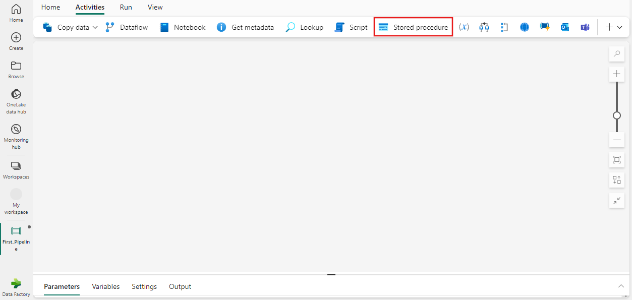
Select Stored Procedure Activity: Within the pipeline, you can add a stored procedure activity by selecting it from the available activities.
Configure the Stored Procedure: After adding the stored procedure activity, you need to configure it by specifying the database, the stored procedure name, and any required parameters.
Notebooks
Notebooks are interactive coding environments that support multiple languages and are used for data exploration, visualization, and complex data transformations.
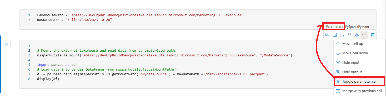
Parameterize the Notebook: If you want to use the notebook as part of a pipeline, you can parameterize it by designating a cell as the parameters cell. This allows the pipeline activity to pass parameters at execution time.
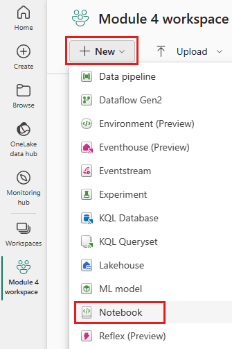
Create a New Notebook: In your workspace, create a new notebook where you can write custom code for data processing tasks.
Add Notebook to Pipeline: Once the notebook is ready, add a new notebook activity to the pipeline and select the notebook you created.
Run the Notebook: Execute the notebook to ensure that the code works as expected and that data is processed correctly.
Dataflows
Dataflows are a series of data transformation steps that prepare data for analysis. They are used to clean, aggregate, and transform data from various sources.
Create a Dataflow: Before adding a dataflow to a pipeline, you need to create one that defines the transformation logic.
Add Dataflow to Pipeline: In the pipeline, add a new dataflow activity and select the previously created dataflow.
Configure the Dataflow: Set up the dataflow by specifying the source, transformation steps, and destination for the data.
Link Activities: If necessary, link the notebook activity to the dataflow activity with a success trigger to ensure that the dataflow runs after the notebook has successfully completed its tasks.
Run the Pipeline: Save your changes and execute the pipeline to process the data according to the defined logic in the stored procedures, notebooks, and dataflows.
For additional information on these topics, you can refer to the following URLs:
- For parameterizing notebooks: Toggle parameter cell https://learn.microsoft.com/en-us/fabric/data-science/../data-engineering/author-execute-notebook .
- For creating and running notebooks: New notebook https://learn.microsoft.com/en-us/fabric/data-factory/tutorial-setup-incremental-refresh-with-dataflows-gen2 .
- For adding stored procedures to a pipeline: Add stored procedure activity https://learn.microsoft.com/en-us/fabric/data-factory/stored-procedure-activity .
- For creating and configuring data pipelines: Create pipeline https://learn.microsoft.com/en-us/fabric/data-factory/tutorial-dataflows-gen2-pipeline-activity .
By integrating these components into a data pipeline, you can automate complex data processing workflows, making them more efficient and reliable.
Prepare and serve data
Copy data
Schedule Data Pipelines
Scheduling data pipelines is an essential aspect of data processing and automation. It allows for the execution of data-related tasks at predefined intervals, ensuring that data is consistently processed and updated without manual intervention. Here’s a detailed explanation of how to schedule data pipelines:
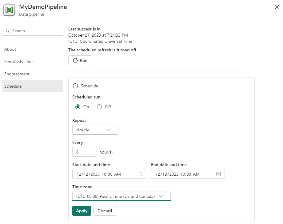
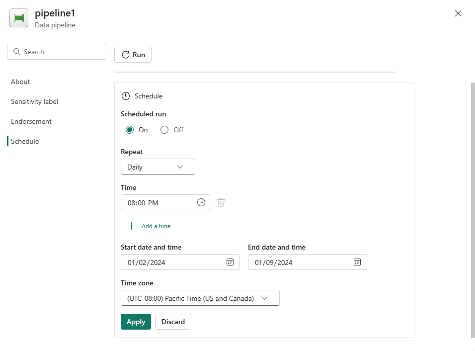
Accessing the Schedule Configuration: To schedule a data pipeline run, navigate to the Home tab of your data pipeline editor and select the Schedule option. This will open the Schedule configuration page https://learn.microsoft.com/en-us/fabric/data-factory/pipeline-runs .
Setting the Schedule Frequency: On the Schedule configuration page, you can define how often your pipeline should run. Options include specific intervals such as daily, hourly, or even every minute. You can also set the exact time for the pipeline to execute https://learn.microsoft.com/en-us/fabric/data-factory/tutorial-dataflows-gen2-pipeline-activity .
Defining Start and End Dates: Specify the start and end dates for your pipeline schedule. This ensures that the pipeline runs within a defined timeframe, which can be particularly useful for pipelines that only need to run during certain periods https://learn.microsoft.com/en-us/fabric/data-factory/tutorial-dataflows-gen2-pipeline-activity .
Choosing the Time Zone: Select the appropriate time zone for your schedule. This is crucial for coordinating pipeline runs with data availability and business processes that may span multiple time zones https://learn.microsoft.com/en-us/fabric/data-factory/tutorial-dataflows-gen2-pipeline-activity .
Applying the Schedule: Once you have configured the schedule settings, select Apply to activate the schedule. Your pipeline will then run automatically according to the specified frequency and time frame https://learn.microsoft.com/en-us/fabric/data-factory/pipeline-runs https://learn.microsoft.com/en-us/fabric/data-factory/tutorial-dataflows-gen2-pipeline-activity .
Monitoring Scheduled Runs: After scheduling your pipeline, you can monitor its execution through the Monitor Hub or by checking the Run history tab in the data pipeline dropdown menu. This allows you to track the status and performance of your scheduled pipeline runs https://learn.microsoft.com/en-us/fabric/data-factory/tutorial-dataflows-gen2-pipeline-activity .
Integration with Workflow Systems: For more complex scheduling and dependency management, workflow systems like Apache Airflow can be used. These systems enable you to define task dependencies, schedule pipeline runs, and monitor workflows effectively https://learn.microsoft.com/en-us/azure/databricks/workflows/jobs/how-to/use-airflow-with-jobs .
Example of Scheduling a Pipeline: An example of scheduling a pipeline could involve setting it to execute daily at a specific time, such as 8:00 PM, and continue to do so until a specified end date, like the end of the year https://learn.microsoft.com/en-us/fabric/data-factory/transform-data .
Scheduling Frequency Options: The frequency of the schedule can be as granular as every few minutes, which is useful for high-frequency data ingestion or processing tasks. You can also define the start and end times for the schedule to control the duration of the recurring runs .
For additional information on scheduling data pipelines, you can refer to the following resources: - Configure a schedule for a pipeline run - Setting a schedule for data pipeline execution - Apache Airflow for managing and scheduling data pipelines - Example of scheduling a pipeline to execute daily - Monitoring the scheduled data pipeline runs
By following these steps and utilizing the provided resources, you can effectively schedule and manage your data pipelines to automate and streamline your data processing workflows.
Prepare and serve data
Copy data
Schedule Dataflows and Notebooks
When working with dataflows and notebooks in Azure, scheduling is a crucial feature that allows for the automation of data processing workflows. Scheduling can be set up to run these workflows at specific intervals, ensuring that data is processed and available when needed without manual intervention.
Scheduling Dataflows
To schedule a dataflow, you would typically follow these steps:
- After developing and testing your dataflow, navigate to the Home tab of the pipeline editor window and select Schedule.
- In the schedule configuration, you can set up the frequency and timing of the pipeline execution. For example, you might schedule the pipeline to run daily at a specific time.
This scheduling capability is part of a broader process that includes creating a dataflow, transforming data, creating a data pipeline using the dataflow, ordering the execution of steps in the pipeline, and copying data with the Copy Assistant https://learn.microsoft.com/en-us/fabric/data-factory/transform-data .
Scheduling Notebooks in Azure Databricks
For Azure Databricks notebooks, the scheduling process is slightly different:
- Click on the Workflows option in the sidebar.
- Click on the job name in the Name column to view the Job details.
- In the Job details panel, click Add trigger and select Scheduled as the Trigger type.
- Define the schedule by specifying the period, starting time, and time zone. You can also use the Show Cron Syntax checkbox to edit the schedule using Quartz Cron Syntax https://learn.microsoft.com/en-us/azure/databricks/getting-started/data-pipeline-get-started .
Additionally, you can schedule a dashboard to refresh at a specified interval by creating a scheduled job for the notebook that generates the dashboard https://learn.microsoft.com/en-us/azure/databricks/notebooks/dashboards .
Scheduling a Notebook Job
To schedule a notebook job to run periodically:
- Click the schedule button at the top right of the notebook.
- In the Schedule dialog, you can choose to run the job manually or on a schedule. If scheduled, you can specify the frequency, time, and time zone.
- Select the compute resource to run the task, and optionally enter any parameters to pass to the job.
- Optionally, specify email addresses to receive alerts on job events https://learn.microsoft.com/en-us/azure/databricks/notebooks/schedule-notebook-jobs .
Fair Scheduling Pools
It’s important to note that all queries in a notebook run in the same fair scheduling pool by default. Scheduler pools can be used to allocate how Structured Streaming queries share compute resources, allowing for more efficient use of the cluster https://learn.microsoft.com/en-us/azure/databricks/structured-streaming/scheduler-pools .
For more detailed information on scheduling and managing notebook jobs in Azure Databricks, you can refer to the following URLs:
- Create and manage scheduled notebook jobs https://learn.microsoft.com/en-us/azure/databricks/getting-started/data-pipeline-get-started https://learn.microsoft.com/en-us/azure/databricks/notebooks/dashboards https://learn.microsoft.com/en-us/azure/databricks/notebooks/schedule-notebook-jobs .
- Quartz Cron Syntax https://learn.microsoft.com/en-us/azure/databricks/getting-started/data-pipeline-get-started .
- Apache fair scheduler documentation https://learn.microsoft.com/en-us/azure/databricks/structured-streaming/scheduler-pools .
By setting up schedules for dataflows and notebooks, you can automate your data processing tasks, making your workflows more efficient and reliable.
Prepare and serve data
Transform data
Implementing a data cleansing process is a critical step in ensuring the quality and reliability of data before it is used for analysis or reporting. Data cleansing, also known as data scrubbing, involves identifying and correcting (or removing) errors and inconsistencies in data to improve its quality. Here is a detailed explanation of the steps involved in a data cleansing process:
Data Cleansing Process
Data Assessment: Begin by evaluating the raw data to identify any inaccuracies, incomplete information, or inconsistencies. This step often involves the use of data profiling tools to gain insights into the data and to understand its structure, content, and quality.
Error Identification: Once the assessment is complete, pinpoint the specific errors and inconsistencies. These could range from simple typos or misspellings to more complex issues like duplicate records or missing values.
Data Correction: After identifying the errors, proceed to correct them. This could involve tasks such as standardizing data formats, correcting misspellings, filling in missing values, or resolving duplicate entries. The goal is to ensure that the data is accurate and consistent.
Data Transformation: Transform the data into a format or structure that is suitable for analysis. This may include converting data types, normalizing data (scaling values to a standard range), or encoding categorical variables into numerical values.
Data Enrichment: Enhance the data by adding new relevant information or by consolidating data from multiple sources. This step can help to fill gaps in the data and to provide a more complete picture.
Data Validation: Validate the cleansed data to ensure that it meets the necessary standards of quality and accuracy. This often involves running validation scripts that check for data integrity and consistency.
Monitoring and Maintenance: Continuously monitor the data quality and perform regular maintenance to prevent the reoccurrence of data quality issues. This includes updating data cleansing routines as new types of errors are identified.
Additional Resources
For more information on data cleansing and related processes, you can refer to the following resources:
Data Cleansing and Transformation: Learn about the importance of data cleansing and the various techniques used to transform raw data into a curated model for analytical reporting https://learn.microsoft.com/en-us/power-bi/guidance/fabric-adoption-roadmap-system-oversight .
End-to-End Data Science Workflow: Explore a comprehensive tutorial that covers the entire data science process, including data cleansing, on Microsoft Fabric https://learn.microsoft.com/en-us/fabric/data-science/tutorial-data-science-introduction .
Data Conversion Flow: Understand the detailed steps involved in data conversion, including data cleansing and enrichment scripts, as part of the implementation phase in data projects https://learn.microsoft.com/en-us/industry/well-architected/financial-services/operational-data-estate .
T-SQL Tools and ETL Processes: Discover how to leverage SQL tools for data cleansing as part of data workflows https://learn.microsoft.com/sql/machine-learning/deploy/modify-r-python-code-to-run-in-sql-server .
Data Preparation Best Practices: Gain insights into best practices for data preparation, including data cleansing, to ensure data correctness and completeness https://learn.microsoft.com/en-us/industry/well-architected/financial-services/operational-data-estate .
Remember, the quality of your data directly impacts the accuracy of your insights and decisions. Therefore, implementing a thorough data cleansing process is essential for any data-driven project.
(Note: URLs for additional information have been included as per the user’s request.)
Prepare and serve data
Transform data
Implementing a Star Schema for a Lakehouse or Warehouse with Type 1 and Type 2 Slowly Changing Dimensions
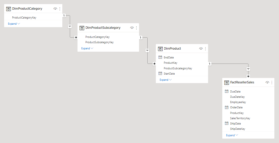
Implementing a star schema in a data lakehouse or warehouse involves organizing data into fact and dimension tables that optimize for query performance and ease of understanding. A star schema is characterized by a central fact table that contains quantitative data, surrounded by dimension tables that contain descriptive attributes related to the facts.
Type 1 Slowly Changing Dimensions (SCDs): Type 1 SCDs are used when it is not necessary to keep track of historical changes in dimension attributes. Instead, when a change occurs, the existing record is updated to reflect the new information. This method is simple and does not require additional storage for historical data. However, it does not preserve historical data, which can be a drawback for certain analyses.
Type 2 Slowly Changing Dimensions (SCDs): Type 2 SCDs, on the other hand, are designed to track historical changes by creating multiple records for a given entity, each with a validity period. This allows for reporting and analysis of data as it changes over time. Implementing Type 2 SCDs typically involves adding columns to track the validity period of each record, such as start and end dates, and a flag to indicate the current record https://learn.microsoft.com/en-AU/azure/cosmos-db/synapse-link-time-travel .
Implementation Steps:
- Design Dimension Tables:
- For Type 1 SCDs, create dimension tables with a surrogate key and include attributes that describe the dimension. When an attribute changes, update the record directly.
- For Type 2 SCDs, add columns to store the validity period of the record (e.g., start date, end date) and a current record flag. When an attribute changes, insert a new record with the updated information and adjust the validity period accordingly https://learn.microsoft.com/en-AU/azure/cosmos-db/synapse-link-time-travel https://learn.microsoft.com/en-us/power-bi/guidance/star-schema .
- Design Fact Table:
- Create a fact table with foreign keys that reference the surrogate keys in the dimension tables. The fact table should contain the measures or quantitative data that will be analyzed https://learn.microsoft.com/en-us/power-bi/guidance/star-schema .
- Data Loading and Transformation:
- Load data into staging tables before transforming it into the star schema format. Use identity columns to keep track of rows during the transformation process https://learn.microsoft.com/en-us/azure/azure-sql/database/saas-tenancy-tenant-analytics-adf .
- For Type 1 SCDs, perform updates directly on the dimension tables.
- For Type 2 SCDs, insert new records into the dimension tables with the appropriate validity period and set the current record flag accordingly https://learn.microsoft.com/en-us/azure/azure-sql/database/saas-tenancy-tenant-analytics-adf .
- Maintain Data Consistency:
- Ensure that dimension tables are loaded before the fact table to maintain referential integrity. This ensures that all referenced dimensions exist when loading facts https://learn.microsoft.com/en-us/azure/azure-sql/database/saas-tenancy-tenant-analytics-adf .
- Use programmatic APIs for delete, update, and merge operations to maintain the data in Delta tables, which can be particularly useful for SCD operations https://learn.microsoft.com/en-us/azure/databricks/archive/runtime-release-notes/6.0 .
- Optimize for Query Performance:
- Design the model to provide tables for filtering, grouping, and summarizing in alignment with star schema principles. This will optimize the performance and usability of the data model, especially when used with tools like Power BI https://learn.microsoft.com/en-us/power-bi/guidance/star-schema .
For additional information on implementing star schemas and managing slowly changing dimensions, you can refer to the following resources: - What is Delta Lake? https://learn.microsoft.com/en-us/azure/databricks/archive/runtime-release-notes/6.0 - Model relationships in Power BI Desktop https://learn.microsoft.com/en-us/power-bi/guidance/star-schema
By following these steps and best practices, you can effectively implement a star schema for a lakehouse or warehouse that supports both Type 1 and Type 2 slowly changing dimensions, facilitating robust data analysis and reporting.
Prepare and serve data
Transform data
Implementing Bridge Tables for a Lakehouse or a Warehouse
Bridge tables are a key component in data warehousing and lakehouse architectures, particularly when dealing with many-to-many relationships between tables. They are used to provide a more efficient and structured way to handle complex relationships between entities in a database.
Understanding Bridge Tables
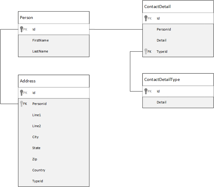
A bridge table, also known as an associative or junction table, is a table that resolves many-to-many relationships between two other tables. It contains the primary keys from each of the two tables, creating a composite primary key for the bridge table itself. This design allows for more flexible and efficient querying and reporting.
Steps to Implement Bridge Tables
Identify Many-to-Many Relationships: Before creating a bridge table, you need to identify the many-to-many relationships within your data model. These are situations where a single record in one table can relate to multiple records in another table and vice versa.
Design the Bridge Table: Once you’ve identified a many-to-many relationship, design a bridge table that includes the primary keys from the related tables. These keys will become foreign keys in the bridge table.
Create the Bridge Table: Using SQL, create the bridge table with the necessary foreign keys and any additional columns that may be required for your specific use case.
CREATE TABLE bridge_table_name (
    foreign_key_to_first_table INT,
    foreign_key_to_second_table INT,
    additional_column1 DATA_TYPE,
    additional_column2 DATA_TYPE,
    ...
    PRIMARY KEY (foreign_key_to_first_table, foreign_key_to_second_table),
    FOREIGN KEY (foreign_key_to_first_table) REFERENCES first_table_name(primary_key_column),
    FOREIGN KEY (foreign_key_to_second_table) REFERENCES second_table_name(primary_key_column)
);
Populate the Bridge Table: Insert data into the bridge table to represent the relationships between the records in the two related tables.
Query Using the Bridge Table: You can now write queries that join the related tables through the bridge table, allowing you to efficiently retrieve data that reflects the many-to-many relationships.
Best Practices
- Normalization: Ensure that your data model is properly normalized to avoid redundancy and maintain data integrity.
- Indexing: Consider indexing the foreign keys in the bridge table to improve the performance of queries that join through the bridge table.
- Data Consistency: Implement constraints and triggers to maintain data consistency across the related tables and the bridge table.
Additional Resources
For more information on implementing bridge tables and best practices in data warehousing and lakehouse architectures, you can refer to the following resources:
- Write a cross-database SQL Query .
- Databricks Lakehouse Architecture https://learn.microsoft.com/en-us/azure/databricks/lakehouse/data-objects .
- Column-level Security in Fabric Data Warehousing https://learn.microsoft.com/en-us/fabric/data-warehouse/tutorial-column-level-security .
- Cross-Workspace Data Analytics https://learn.microsoft.com/en-us/fabric/data-warehouse/get-started-lakehouse-sql-analytics-endpoint .
By following these guidelines and utilizing the provided resources, you can effectively implement bridge tables in your lakehouse or warehouse to manage complex data relationships and enhance your data analytics capabilities.
Prepare and serve data
Transform data
Denormalize Data
Denormalization is a database optimization technique where redundant data is added to one or more tables. This can improve the performance of read queries by reducing the need for joins and aggregations. However, it can lead to increased storage costs and more complex update operations.
Advantages of Denormalization:
- Improved Query Performance: By storing summary entities or pre-joined data, queries can access all the required information from a single entity, which can be significantly faster than executing multiple joins across several tables https://learn.microsoft.com/en-AU/azure/storage/tables/table-storage-design-guidelines .
- Simplified Queries: Denormalization can simplify the structure of queries, making them easier to write and understand, especially when dealing with aggregate data https://learn.microsoft.com/en-AU/azure/storage/tables/table-storage-design-guidelines .
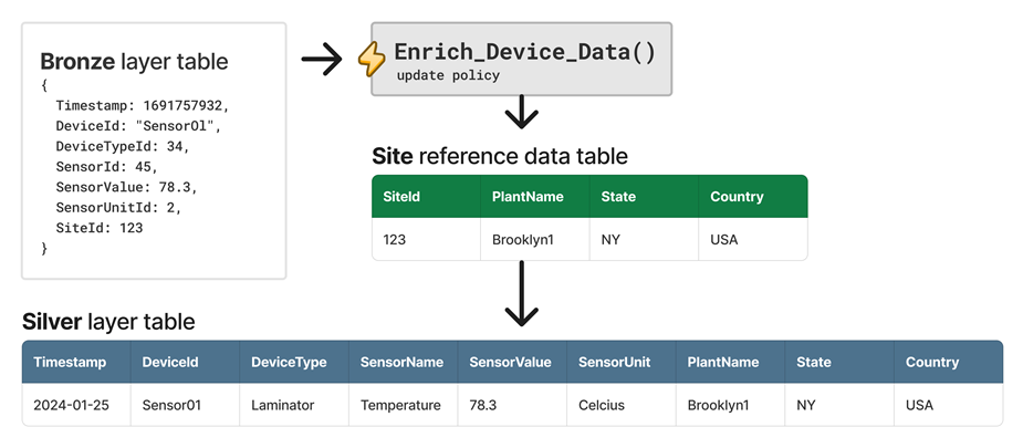
- Efficient Data Ingestion: When data is denormalized at ingestion time, the computational cost of joins is reduced because they operate on a smaller batch of data. This can greatly enhance the performance of downstream queries https://learn.microsoft.com/azure/data-explorer/kusto/management/update-policy-common-scenarios .
Considerations for Denormalization:
- Increased Storage Costs: Since denormalization involves storing additional copies of data, it can lead to higher storage costs .
- Complex Updates: When data is denormalized, updates may need to be propagated to multiple places, which can complicate update operations https://learn.microsoft.com/en-AU/azure/cosmos-db/nosql/modeling-data .
- Data Redundancy: Denormalization can lead to data redundancy, which might result in data inconsistency if not managed properly .
Examples of Denormalization:
- Azure Cosmos DB: In Azure Cosmos DB, entities are treated as self-contained items represented as JSON documents. Data is denormalized by embedding all related information into a single document, which can result in fewer queries and updates to complete common operations https://learn.microsoft.com/en-AU/azure/cosmos-db/nosql/modeling-data .
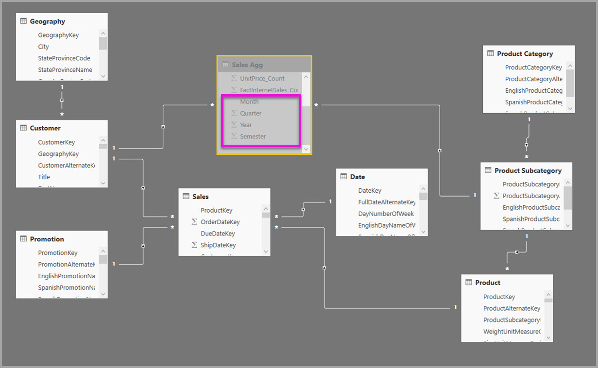
- Snowflake Dimension: In a snowflake dimension design, related tables are normalized and positioned outwards from the fact table, forming a snowflake design. However, integrating these tables into a single model table (denormalization) can offer benefits such as improved performance and a more intuitive experience for report authors https://learn.microsoft.com/en-us/power-bi/guidance/star-schema .
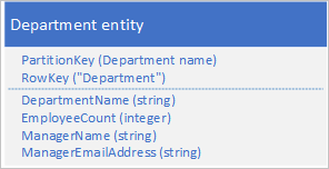
- Azure Table Storage: In Azure Table Storage, denormalizing data can involve keeping a copy of related information, such as a manager’s details, within the department entity. This allows for retrieving all necessary details with a point query https://learn.microsoft.com/en-AU/azure/storage/tables/table-storage-design-patterns .
For additional information on denormalization and its implications, you can refer to the following resources: - Star Schema Design - Optimize Data Models - Modeling Data in Azure Cosmos DB - Snowflake Design in Power BI - Azure Storage Table Design Guide
Please note that while denormalization can offer performance benefits, it is important to carefully consider the trade-offs and ensure that it aligns with the specific requirements and constraints of your data model.
Prepare and serve data
Transform data
Aggregate or De-aggregate Data
Aggregating data refers to the process of summarizing or combining data from detailed data sets to create totals or summary information. De-aggregating data, on the other hand, involves breaking down aggregated data into its individual components or more detailed data.
Aggregation Techniques:
Using Spark SQL for Aggregation:
- Spark SQL can be utilized to perform joins and aggregate functions on data, which is particularly beneficial for individuals with a SQL background transitioning to Spark. This method involves creating Spark dataframes from existing delta tables, performing joins, grouping by certain columns to generate aggregates, and then writing the results as a delta table to persist the data https://learn.microsoft.com/en-us/fabric/data-engineering/tutorial-lakehouse-data-preparation .
Example Code Snippet:
df_fact_sale = spark.read.table("wwilakehouse.fact_sale")
df_dimension_date = spark.read.table("wwilakehouse.dimension_date")
df_dimension_city = spark.read.table("wwilakehouse.dimension_city")

sale_by_date_city = df_fact_sale.alias("sale") \
    .join(df_dimension_date.alias("date"), df_fact_sale.InvoiceDateKey == df_dimension_date.Date, "inner") \
    .join(df_dimension_city.alias("city"), df_fact_sale.CityKey == df_dimension_city.CityKey, "inner") \
    .groupBy("date.Date", "city.City") \
    .sum("sale.TotalExcludingTax", "sale.Profit") \
    .withColumnRenamed("sum(TotalExcludingTax)", "SumOfTotalExcludingTax") \
    .orderBy("date.Date", "city.City")
sale_by_date_city.write.mode("overwrite").format("delta").save("Tables/aggregate_sale_by_date_city")
Using Spark SQL Temporary Views:
- Temporary Spark views can be created to join tables and perform aggregations. This approach is similar to the previous one but uses Spark SQL syntax to create and manipulate the data https://learn.microsoft.com/en-us/fabric/data-engineering/tutorial-lakehouse-data-preparation .
Example Code Snippet:
CREATE OR REPLACE TEMPORARY VIEW sale_by_date_employee AS
SELECT DD.Date, DD.CalendarMonthLabel, SUM(FS.TotalExcludingTax) SumOfTotalExcludingTax
FROM wwilakehouse.fact_sale FS
INNER JOIN wwilakehouse.dimension_date DD ON FS.InvoiceDateKey = DD.Date
GROUP BY DD.Date, DD.CalendarMonthLabel
ORDER BY DD.Date ASC
Type Conversion for Aggregation:
- When aggregating data with different numeric data types, it is
necessary to convert them to a consistent data type using functions like
CInt,CDbl, orCDechttps://learn.microsoft.com/en-us/power-bi/create-reports/../paginated-reports/expressions/report-builder-functions-varp-function .
For more information on type conversion functions, refer to the Type Conversion Functions documentation.
- When aggregating data with different numeric data types, it is
necessary to convert them to a consistent data type using functions like
Handling Aggregations with Different Storage Modes:
- When combining DirectQuery, Import, and Dual storage modes, it is crucial to keep the in-memory cache in sync with the source data to ensure accurate aggregation results https://learn.microsoft.com/en-us/power-bi/transform-model/aggregations-advanced .
Server Aggregates:
- The
Aggregatefunction can be used to display aggregates calculated on the external data source. This is supported by certain data extensions and is particularly relevant when using SQL Server Analysis Services https://learn.microsoft.com/en-us/power-bi/create-reports/../paginated-reports/expressions/report-builder-functions-aggregate-function .
For more information on server aggregates, refer to the Analysis Services MDX Query Designer User Interface (Report Builder) documentation.
- The
Combining Relationships and GroupBy Columns:
- Aggregations can be optimized by combining relationships and GroupBy columns. This may involve replicating certain attributes in the aggregation table and using relationships for others https://learn.microsoft.com/en-us/power-bi/transform-model/aggregations-advanced .
For more information on advanced aggregation techniques, refer to the Aggregations in Power BI documentation.
De-aggregation Techniques:
De-aggregation is less common as a process but can be necessary when detailed data is required from summary information. This can involve distributing aggregated totals based on certain proportions or assumptions, or simply accessing the underlying detailed data that was used to create the aggregate.
In summary, aggregation and de-aggregation are essential techniques in data preparation and analysis, allowing for the transformation of data into meaningful insights. The choice of method depends on the specific requirements of the analysis and the background of the data professional.
Prepare and serve data
Transform data
Merge or Join Data
Merging or joining data is a fundamental operation in data processing that combines rows from two or more tables based on a related column between them. This operation is essential when you need to consolidate data from different sources or when you want to enrich a dataset with additional attributes.
Merge Data
Merging data typically refers to the operation of combining two
datasets into a single dataset. In the context of Azure Data Services,
you can perform an upsert operation using the
MERGE command. This is particularly useful when you need to
update existing data while appending new data to your target table. When
your target table is partitioned, applying a partition filter during the
merge operation can significantly speed up the process by allowing the
engine to eliminate partitions that do not require updating https://learn.microsoft.com/en-us/fabric/onelake/onelake-medallion-lakehouse-architecture
.
For more information on the MERGE command, you can refer
to the official documentation: MERGE
command https://learn.microsoft.com/en-us/fabric/onelake/onelake-medallion-lakehouse-architecture
.
Join Data
Joining data involves combining rows from two or more tables based on a common field. There are various types of joins, such as inner join, outer join, left join, and right join, each serving a different purpose depending on the desired outcome.
For instance, if you want to create a list of states where both
lightning and avalanche events occurred, you can use an inner join to
combine the rows of two tables—one with lightning events and the other
with avalanche events—based on the State column. This will
result in a dataset that includes only the states where both event types
have occurred https://learn.microsoft.com/azure/data-explorer/kusto/query/tutorials/join-data-from-multiple-tables
.
Here is an example query that demonstrates this operation:
StormEvents | where EventType == "Lightning" | distinct State
| join kind=inner (
    StormEvents | where EventType == "Avalanche" | distinct State
) on State
| project State
For more details on how to run this query, visit: Run the query https://learn.microsoft.com/azure/data-explorer/kusto/query/tutorials/join-data-from-multiple-tables .
Filter Data
In Azure Table Storage, you can filter the rows returned from a table
by using an OData style filter string with the
query_entities method. For example, to get all weather
readings for Chicago between two specific dates and times, you would use
a filter string like this:
PartitionKey eq 'Chicago' and RowKey ge '2021-07-01 12:00 AM' and RowKey le '2021-07-02 12:00 AM'You can construct similar filter strings in your code to retrieve data as required by your application https://learn.microsoft.com/en-AU/azure/storage/tables/../../cosmos-db/table-storage-how-to-use-python .
For additional information on OData filter operators, you can visit the Azure Data Tables SDK samples page: Writing Filters https://learn.microsoft.com/en-AU/azure/storage/tables/../../cosmos-db/table-storage-how-to-use-python .
Adaptive Query Execution
In the context of Azure Databricks, Adaptive Query Execution (AQE) is a feature that enhances the performance of join operations. AQE dynamically optimizes query plans by changing join strategies, coalescing partitions, handling skewed data, and propagating empty relations. This results in improved resource utilization and cluster throughput https://learn.microsoft.com/en-us/azure/databricks/optimizations/aqe .
For more information on AQE and its features, you can refer to the Azure Databricks documentation.
By understanding and utilizing these data merging and joining techniques, you can effectively manage and analyze large datasets, leading to more insightful outcomes.
Prepare and serve data
Transform data
Identifying and Resolving Duplicate Data, Missing Data, or Null Values
When working with data, it is crucial to ensure the accuracy and consistency of the dataset. Identifying and resolving issues such as duplicate data, missing data, or null values is an essential step in data preparation and cleaning. Here’s a detailed explanation of how to address these common data issues:
Duplicate Data
Duplicate data can lead to skewed results and inaccurate analyses. To handle duplicates, you can define a function that removes duplicate rows based on specific columns. For instance, if you have a dataset with customer information, you might want to remove entries that have the same customer ID and row number:
def clean_data(df):
    # Drop duplicate rows based on 'RowNumber' and 'CustomerId'
    df = df.dropDuplicates(subset=['RowNumber', 'CustomerId'])
    return df
This function will ensure that each customer is represented only once in your dataset https://learn.microsoft.com/en-us/fabric/data-science/how-to-use-automated-machine-learning-fabric .
Missing Data
Missing data, or null values, can occur for various reasons, such as errors during data collection or transfer. To handle missing data, you can drop rows that have null values across all columns or specific columns that are critical for your analysis:
def clean_data(df):
    # Drop rows with missing data across all columns
    df = df.dropna(how="all")
    return df
This approach will remove any rows that do not contain any data, thus cleaning your dataset https://learn.microsoft.com/en-us/fabric/data-science/how-to-use-automated-machine-learning-fabric .
Null Values
Null values can also be indicative of missing information and need to be addressed. Depending on the context, you might choose to fill null values with a default value, use interpolation methods to estimate the missing value, or simply remove the rows or columns with too many nulls.
For handling missing values in delimited text files, especially when
using PolyBase, you can specify how to handle these missing values. The
Use type default property allows you to define the behavior
for missing values when retrieving data from the text file https://learn.microsoft.com/en-us/fabric/data-factory/connector-azure-synapse-analytics-copy-activity
.
Additional Resources
For more information on handling data uniqueness and ensuring data accuracy, you can refer to the following resources: - Primary key evaluation rule for setting up record uniqueness in Microsoft Sustainability Manager https://learn.microsoft.com/en-us/industry/well-architected/sustainability/sustainability-manager-data-traceability-design . - CREATE EXTERNAL FILE FORMAT (Transact-SQL) for understanding how to handle missing values in text files when using PolyBase https://learn.microsoft.com/en-us/fabric/data-factory/connector-azure-synapse-analytics-copy-activity .
By following these guidelines and utilizing the provided resources, you can effectively identify and resolve issues with duplicate data, missing data, or null values, ensuring a clean and reliable dataset for analysis.
Prepare and serve data
Transform data
Convert Data Types Using SQL or PySpark
When working with data in SQL or PySpark, it is often necessary to convert data types to ensure compatibility and proper functioning of operations. Here’s a detailed explanation of how to convert data types in both SQL and PySpark environments.
SQL Data Type Conversion
In SQL, data type conversion can be achieved using the
CAST or CONVERT function. These functions
allow you to change a value from one data type to another. For example,
to convert a column of type VARCHAR to an INTEGER, you would use the
following SQL statement:
SELECT CAST(column_name AS INT) FROM table_name;Or using the CONVERT function:
SELECT CONVERT(INT, column_name) FROM table_name;It’s important to note that while SQL Server supports a wide range of data types, implicit conversions might occur when using data from SQL Server in other environments, such as R scripts. If an exact conversion cannot be performed automatically, an error may be returned https://learn.microsoft.com/sql/machine-learning/r/r-libraries-and-data-types .
PySpark Data Type Conversion
In PySpark, data type conversion can be performed using the
withColumn method along with the cast function
from the pyspark.sql.functions module. For instance, to
change the data type of a column named churn from Boolean
to Integer, you would use the following PySpark code:
from pyspark.sql.functions import col

df = df.withColumn("churn", col("churn").cast("integer"))
The Databricks Assistant suggests providing more detail in your prompts to get the most accurate answer, such as specifying if column data type conversions are needed https://learn.microsoft.com/en-us/azure/databricks/notebooks/use-databricks-assistant .
For additional information on PySpark data type conversions and interoperability between PySpark and pandas, you can refer to the following resources:
- Pandas Function APIs: [https://learn.microsoft.com/en-us/azure/databricks/pandas/pandas-function-apis] https://learn.microsoft.com/en-us/azure/databricks/reference/api
- Convert between PySpark and pandas DataFrames: [https://learn.microsoft.com/en-us/azure/databricks/pandas/pyspark-pandas-conversion] https://learn.microsoft.com/en-us/azure/databricks/reference/api
Additional Resources
For more detailed instructions on creating a PySpark notebook and importing the necessary types for data type conversion, you can visit the following link:
- Create a notebook: [https://learn.microsoft.com/en-us/fabric/data-science/data-engineering/how-to-use-notebook] https://learn.microsoft.com/en-us/fabric/data-science/model-training/fabric-sparkml-tutorial
When converting data types, it is essential to ensure that the target data type is supported by the destination environment. For example, when moving data from Python to SQL, you may need to convert the data types to those supported by SQL https://learn.microsoft.com/azure/azure-sql-edge/deploy-onnx .
By understanding and utilizing these conversion techniques, you can effectively manage and manipulate data types within SQL and PySpark, ensuring that your data is in the correct format for analysis and processing.
Prepare and serve data
Transform data
Filter Data in Power BI
Filtering data in Power BI is a crucial skill for uncovering insights and making the most of the data visualizations. Power BI provides a variety of ways to filter data, both before and after it has been loaded into a report.
Before Data Loading
Query Filters: When you want to reduce the amount of data retrieved and processed in a report, you can change the query for each dataset. This is done at the data source level and is an efficient way to handle large datasets https://learn.microsoft.com/en-us/power-bi/create-reports/../paginated-reports/report-design/add-dataset-filters-data-region-filters-and-group-filters .
PowerShell Scripting: For more advanced users, PowerShell scripts can be used to retrieve data from the activity log using the Power BI Management module. These scripts can be adapted for production by adding logging, error handling, alerting, and refactoring for code reuse https://learn.microsoft.com/en-us/power-bi/guidance/admin-activity-log .
After Data Loading
Report Filters: If you cannot filter data at the source, you can specify filters for report items. Filter expressions can be set for a dataset, a data region, or a group within the report. Parameters can also be included in filter expressions to filter data for specific values or users https://learn.microsoft.com/en-us/power-bi/create-reports/../paginated-reports/report-design/add-dataset-filters-data-region-filters-and-group-filters .
Filters Pane: The Filters pane in the Power BI service allows you to apply filters to your reports. You can filter data by selecting data points on a report visual, which then filters other visuals on the page through cross-filtering and cross-highlighting https://learn.microsoft.com/en-us/power-bi/consumer/end-user-report-filter .
Insights Feature: The Insights feature in Power BI can automatically find anomalies and trends in your data. However, it has certain limitations, such as not being available in apps and embedded for reports in Premium workspaces, and it does not support certain data types and functionalities https://learn.microsoft.com/en-us/power-bi/create-reports/insights .
Considerations
- Some data or visuals may not be supported by the Insights feature, such as custom date hierarchies or non-numeric measures https://learn.microsoft.com/en-us/power-bi/create-reports/insights .
- Explanations provided by Insights are not supported in cases of TopN filters, include/exclude filters, measure filters, and certain measure types https://learn.microsoft.com/en-us/power-bi/create-reports/insights .
- It is recommended to keep scripts for extracting data as simple as possible, following an ELT methodology (Extract, Load, Transform) https://learn.microsoft.com/en-us/power-bi/guidance/admin-activity-log .
For more information on how visuals cross-filter each other in a Power BI report, you can visit the following URL: How visuals cross-filter each other in a Power BI report.
By understanding and utilizing these filtering techniques, you can effectively manage and analyze your data within Power BI, leading to more meaningful insights and a more powerful reporting experience.
Prepare and serve data
Transform data
Filter Data in Power BI
Filtering data in Power BI is a crucial skill for designing effective reports and gaining insights from the data. Power BI provides several methods to filter data, each suitable for different scenarios and requirements.
Report Filters Pane
The Filters pane in Power BI allows users to apply filters to reports at various levels:
- Visual-level filters apply to a single visual on a report page.
- Page-level filters apply to all visuals on a report page.
- Report-level filters apply to all visuals across all pages in the report.
Filters can be based on fields, values, or date ranges, and they can be used to include or exclude data points. For more information on using the Filters pane, refer to the Power BI documentation on filtering here https://learn.microsoft.com/en-us/power-bi/consumer/end-user-report-filter .
Cross-filtering and Cross-highlighting
Cross-filtering and cross-highlighting are interactive features that allow users to click on data points in one visual to filter or highlight related data in other visuals on the same report page. This interactivity provides a dynamic way to explore and drill down into data. For a detailed explanation of how visuals cross-filter each other in a Power BI report, see the Microsoft documentation here https://learn.microsoft.com/en-us/power-bi/consumer/end-user-report-filter .
Filtering Data at the Source
When possible, it’s efficient to filter data at the data source level. This can be done by modifying the query that retrieves the data. Filtering at the source reduces the amount of data that needs to be processed in the report, which can improve performance. For more information on filtering at the source, see the guidance provided here https://learn.microsoft.com/en-us/power-bi/create-reports/../paginated-reports/report-design/add-dataset-filters-data-region-filters-and-group-filters .
Filtering Data After Loading
In cases where filtering at the source is not possible, Power BI allows for filtering data after it has been loaded into the report. This can be done by creating filter expressions for datasets, data regions, or groups within the report. Parameters can also be included in filter expressions to allow for dynamic filtering based on user input or other criteria https://learn.microsoft.com/en-us/power-bi/create-reports/../paginated-reports/report-design/add-dataset-filters-data-region-filters-and-group-filters .
Insights and Limitations
Power BI’s Insights feature can automatically find patterns, trends, and anomalies in the data. However, there are limitations to where Insights can be used and the types of data it supports. For instance, Insights does not work with non-numeric measures or custom date hierarchies. Additionally, certain functionalities like Publish to Web and Live Connection to certain data sources are not supported with Insights https://learn.microsoft.com/en-us/power-bi/create-reports/insights .
PowerShell Scripting for Activity Data
For more advanced users, Power BI Management PowerShell module can be used to retrieve data from the activity log. This is particularly useful for administrators or developers who need to automate the extraction of activity data for analysis or monitoring. The scripts provided in the documentation are for educational purposes and may need to be adapted for production use https://learn.microsoft.com/en-us/power-bi/guidance/admin-activity-log .
By understanding and utilizing these filtering techniques, users can create more focused and insightful Power BI reports. Remember to review the Power BI documentation for the most up-to-date information and best practices.